
By Jonathan Fula, Karim Jacquelin, FIS – APTimum, Mila Sherman, and Kristen Walters, CISDM Advisory Board, Isenberg School of Management, UMASS Amherst and Center for International Securities and Derivatives Markets (CISDM)
1. Stress Test Scenarios and Endowment Portfolio Impacts
1.1 Forward Looking Stress Scenarios
Global markets face several correlated risks that could drive large, multi-variate market reversals. These scenarios share common drivers: inflation and interest rates. This section presents four forward-looking scenarios that estimate how a market reversal could spread across financial markets. The first three are geopolitical scenarios linked to a single Middle East trajectory, ordered by the extent of the disruption and number of financial market channels affected. The fourth does not depend on a geopolitical or energy shock and shows that the same rate-driven market damage could occur without a continued Strait closure or other Middle East disruptions.
As of the August 14th baseline the US-Iran conflict remained unresolved, Hormuz shipping was severely constrained, and Houthi activity had already escalated risk in the Red Sea and Bab al-Mandab. The June interim agreement expired on August 17th without restoring normal maritime flows, so energy disruption and inflationary consequences were already embedded in market prices.
- Middle East Escalation. Scenario extends the current conflict into a prolonged, more severe Hormuz disruption with effects on secondary chokepoints. Supply pressure that began in crude and distillates spreads to LNG, ethanol, fertilizer, aluminum, petrochemicals, feedstocks and food, feeding through to rates, credit and equities. The AI complex stays comparatively decoupled on continued hype and elevated valuations.
- Continued Escalation with AI De-rating. The scenario applies the same oil shock but intensifies the rate channel. Sustained closure keeps core inflation elevated which keeps the Fed restrictive. Higher policy rates lift the entire rate curve, and a higher discount rate compresses the multiples of long-duration growth names with values extending far in the future. The AI trade affects markets through rates rather than earnings.
- Extreme Escalation. This is the regional-system tail scenario. It layers moves from recurring Red Sea attacks toward sustained closure of Bab al-Mandab, plus damage to non-Iranian Gulf producer infrastructure, on top of the Hormuz closure. This removes the spare capacity that could potentially backfill the shortfall. Each independent leg is damaging and collectively the impact results in a market with no relief valve.
- FED Trap / Persistent Inflation. This scenario is not directly related to escalation in the Middle East. The scenario captures any persistent core inflation impulse (fiscal, tariffs, wages) that keeps the Fed restrictive and long rates high with the same market same damage. The scenario is based on how high core PCE runs (4.5%, 5%, 6%) and for how long (3 to 24 months). Growth is not an explicit input, so the scenario turns fully stagflationary only at longer horizons where recession risk increases.
1.2 Macroeconomic Indicators and Policy Variables
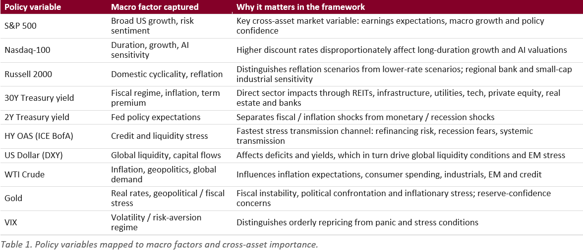
The methodology first identifies the macroeconomic indicators each scenario affects, then selects a small set of policy variables directly impacted by those indicators, and projects those shocks onto statistical factors. Propagation to all other assets and portfolios is implied by factor sensitivities, which capture cross-asset co-movement. All four scenarios from a US investor perspective on the same macro-factor and policy-variable set.
1.3 Baseline Levels, 14 August 2026

These starting levels affect everything downstream. The front end is not neutral. The oil curve is backwardated, so spot prices carry a near-term war premium while deferred futures imply almost none. Gold, which is near a record level, and a firm dollar both indicate haven demand before any scenario unfolds.
It is worth noting how thinly that premium is priced. Multiple dealer estimates put oil at $140 to $180 or higher on a continued Strait closure, with global inventories at roughly 45-year lows relative to demand and no clear path to resolution. The gap reflects several factors, particularly Chinese demand destruction, and suggests crude is being influenced by behavioral factors as much as fundamentals. The implication is that the market may be underpricing the oil leg that drives all three geopolitical tails.
2. Tail Scenario Results
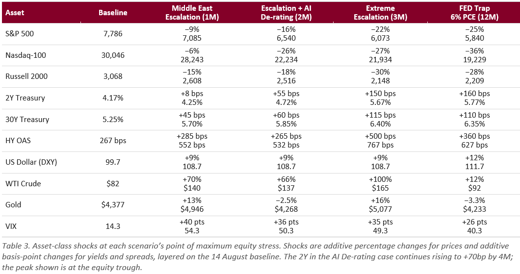
The table below consolidates all four scenarios at points of maximum equity stress. The three geopolitical scenarios peak and retrace, and peak progressively later as severity rises: Middle East Escalation at one month, AI De-rating at two, Extreme Escalation at three. The FED Trap does not retrace and shown at 12 months in the 6% core PCE regime.
2.1 Scenario Amplification and Escalation
Middle East Escalation. The base case disruption produces a substantially larger and more persistent oil shock than markets currently price. WTI rises 70% to roughly $140 in month one and remains about 50% above baseline five months later. Persistence raises inflation pressure, widens credit, lifts long yields and strengthens haven demand for both gold and the dollar. The Nasdaq is comparatively resilient at −6% because the long-duration technology complex has not yet experienced the rate-driven de-rating.
Escalation with AI De-rating. This scenario isolates an incremental increase in rates with the oil path, credit widening, dollar and VIX essentially unchanged from the scenario above. With higher rates, the Nasdaq falls -26% at the trough rather than -6%, the 2-year rises +70 bps rather than staying level, the S&P drawdown deepens from −9% to −16%, and gold reverses lower as the rate shock dampens haven support. The incremental damage comes not from a bigger shock but from the same trigger flowing through rates which is why a portfolio hedged on oil outcomes alone can still perform poorly.
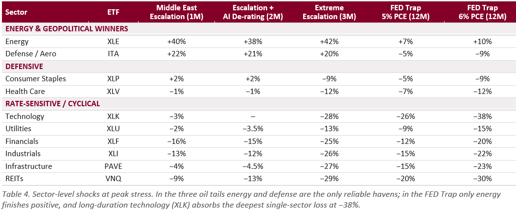
Extreme Escalation. Under this scenario, three things happen at once with elements of all three visible today. This includes sustained Hormuz closure, escalation of ongoing Red Sea attacks into closure of Bab al-Mandab, and damage to non-Iranian Gulf producer infrastructure. The calibration is anchored to outside estimates, such as JPMorgan’s June 2026 update estimating Brent at $120 to 130 near term and above $150 on persistence, with the wider Street running to $200. The central path peaks at WTI near $165 (Brent near $170), inside that range rather than at its extreme. The distinguishing feature is the front end of the yield curve. The 2-year rises +150 bps to 5.67% which implies a terminal policy rate near 5.5 to 6.0% against the 3.5 to 3.75% baseline. In an ordinary recession the Fed cuts and the front-end rallies, but in this case, the Fed must tighten into the growth shock. The 30-year sells off 115 bps alongside equities, so duration hedges underperform. Only energy and defense finish positive within equities. Cross-asset protection comes from gold or an outright short in duration.
FED Trap / Persistent Inflation. This scenario is structurally different from the first three and not linked to oil or geopolitics. Persistent core inflation can arise from fiscal deficits, issuance levels, tariffs or wage growth; what matters is the consequence. At 4.5% core PCE the S&P falls -8% over twelve months and the 2-year rises +30 bps which is uncomfortable but manageable. At 5% the S&P falls -16% and the 2-year rises +90 bps. At 6%, closest to realized 2022, the S&P falls -25%, the 2-year rises +160 bps and high-yield spreads more than double. Across all three regimes the defining risk is identical: equities and the bond hedge decline together, driven by inflation rather than growth as the central bank’s binding constraint. Damage deepens rather than retraces and the 6% regime runs from −21.2% for the S&P at six months to −31.2% at twenty-four. The MOVE index is shown as a supplemental bond-volatility measure (rising to 168 at 12M in the 6% regime) and is not one of the ten core policy variables.
2.2 Sector Dispersion at Peak Stress
3. Historical Calibration and Plausibility
3.1 Calibration against realized crises
By design, each scenario is calibrated to keep market moves inside a previously observed historical range where one exists. The 100% oil move in Extreme Escalation looks outsized until compared against the dot-com-era precedent, where crude rose more than 200% off a low base, and against 2022, which it exceeds by only about 1.6 times. The most aggressive oil assumption in the entire study is below the worst of the last thirty-five years.
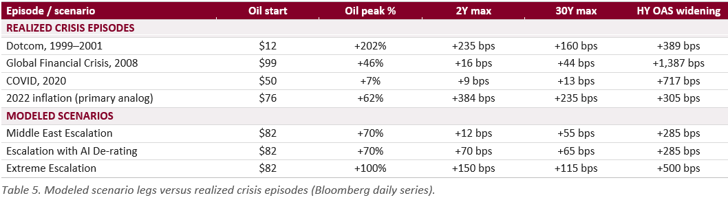
Credit and rates are treated the same way. High-yield widening of +500 bps in the Extreme case sits between 2022 (about +305 bps) and COVID (about +717 bps) and well below 2008 (nearly +1,400 bps), which makes it a severe but non-systemic credit event rather than a full financial crisis. Rate shocks were set deliberately inside crisis precedents rather than at them. The dot-com episode involved the 2-year rising +235 bps from a 4.56% starting level which is close to today’s baseline of 4.17% and therefore a reasonable benchmark with the +150 bps move in the Extreme Escalation scenario significantly lower.
Against the WTI futures strip the divergence is deliberate and explicit. The forward curve is backwardated and prices essentially no sustained war premium, sliding from $82 front-month to $77 by January 2027 and to $55–$65 in the long-dated contracts out to 2037. The Extreme path runs 73% to 106% above the strip at each horizon from one to five months. Every scenario is a considered departure from what the market itself is pricing.
3.2 Method: Scaled Mahalanobis Distance
Scenario tables estimate market moves but do not note whether the combinations of moves are historically unusual. Two scenarios can both look severe while one sits well inside historical experience and the other far outside it. The Mahalanobis distance measures how far a scenario’s shock vector lies from the center of the historical risk-factor distribution while accounting for each factor’s volatility and for the correlations among factors. If oil and rates are historically positively correlated, a scenario in which both move sharply together scores a lower distance than an otherwise identical scenario that ignores that correlation. The analysis uses the scaled distance, divided by the number of risk factors, so results stay comparable across factor sets of different size.
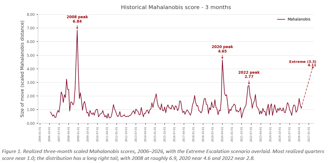
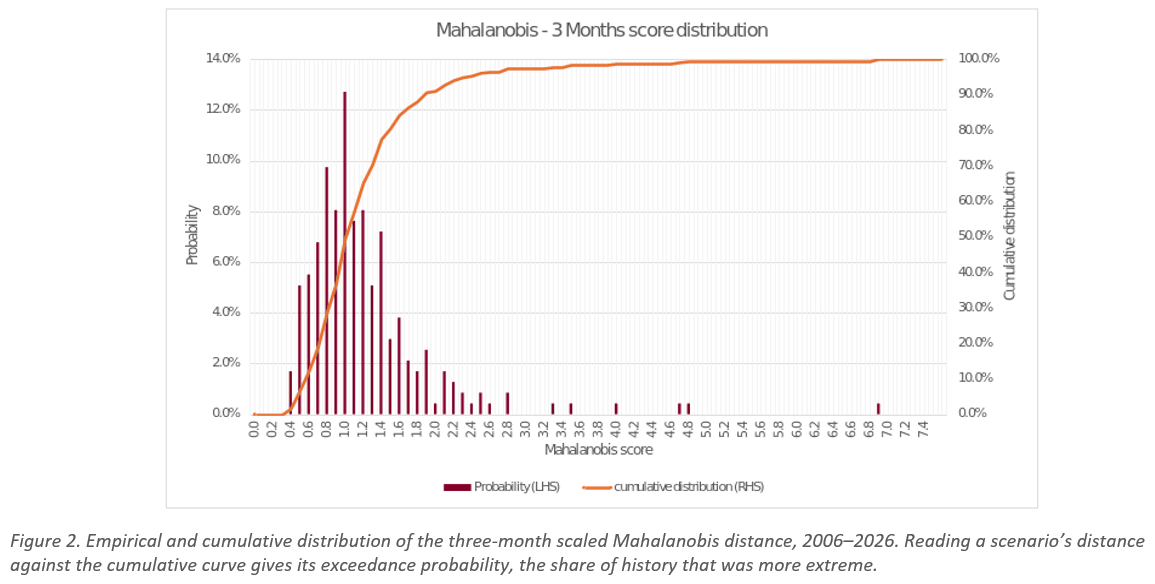
The empirical distribution is built from twenty years of factor returns (June 2006 to June 2026). Rather than using a single covariance matrix over the full sample, each historical observation uses a rolling three-year window. Thus, every score reflects the volatility and correlation structure prevailing at the time. Separate matrices are estimated for each scenario horizon, since both volatility and cross-factor correlation evolve as horizons lengthen. Results are assessed non-parametrically against the realized distribution rather than an assumed one. The three-month horizon is used throughout because it is common to all four scenarios.
3.3 Where the Scenarios Fall

The ranking now carries a probability alongside a distance. Middle East Escalation at 1.27 is a bad but far from unprecedented quarter, exceeded roughly 35% of the time. Adding the AI de-rating channel lifts the score to 2.05, exceeded only 9% of the time, as the rate and technology channels switch on together. Extreme Escalation at 4.11 is a near-record event, exceeded just 1% of the time across twenty years. The FED Trap appears more moderate at a single three-month point (0.67 at 5% core PCE and 1.45 at 6%) because the damage accumulates over a full year rather than as a one quarter’s shock and the three-month score understates a tail that compounds. The scenarios most relevant are the ones the market is not pricing which are the AI de-rating tail and the extreme escalation.
One structural point helps explain why oil-driven scenarios score as extreme sooner. Crude’s annualized factor volatility in the 2006-onward backtest is 36.3%, far above the Russell 2000 at 20.1%, gold at 18.2%, the Nasdaq-100 at 18.1%, the S&P 500 at 13.0%, the dollar at 6.3% and US high yield at 4.1%. A given percentage move in crude therefore represents far fewer standard deviations than the same move elsewhere. Thus, it takes a much larger oil move to reach the same statistical extremity which is the main reason the oil tails dominate the distance analysis.
4. Portfolio Impact: Model Portfolios and US Endowments
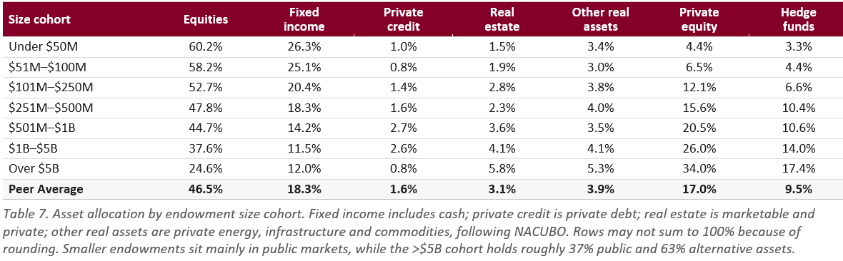
The same ten policy-variable shocks are propagated through the FIS multi-asset class statistical factor model across each investor type’s asset allocation. Scenarios are applied instantaneously to a set of public equity-bond model portfolios and to roughly 650 US college and university endowment funds representing about $900 billion in assets, based on anonymized fund data reported to NACUBO. Because endowment holdings data are not publicly available, granular asset allocation data was mapped to representative public and private market indices.
4.1 Endowment Asset Allocation by Size Cohort
4.2 Methodology Note
Measuring risk consistently across public and private holdings requires normalizing private asset data to the valuation frequency and pricing behavior of public markets. Private assets are appraisal-priced on a lag; public assets mark daily. In the FIS model, private asset risk is measured using de-smoothed private returns, and valuation frequency is adjusted to weekly using synthetic public assets with the same risk profile. Consequently, these results deliberately do not reflect the valuation smoothing and reporting lag that occur in practice for private assets.
Results should be interpreted as factor-based estimates of potential outcomes under specified scenarios, not as predictions. They assume historical relationships among risk factors remain broadly representative and that allocations remain unchanged over the stress horizon. The results are conditional on the modeled scenarios occurring and are not estimates of the probability that those scenarios occur.
4.3 Peak Losses by Scenario
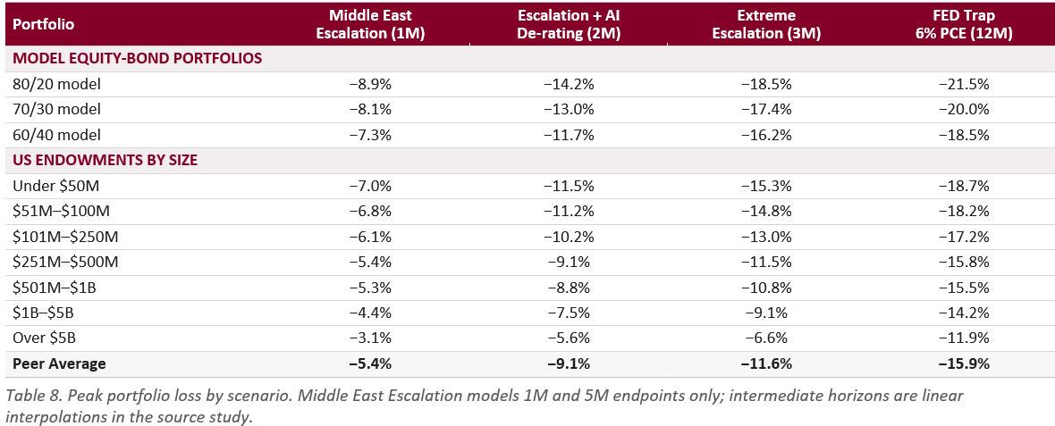
All four scenarios involve an inflationary regime and higher rates, so the historical diversification benefit of holding bonds against equities is lost as the two asset classes become positively correlated. The model equity-bond portfolios therefore incur largest losses in every scenario, and the 60/40 loses more than the 80/20 relative to its equity weight because the fixed income sleeve adds to the loss rather than offsetting it. Endowments perform better despite still-high systematic equity risk, with losses falling monotonically as fund size rises, because larger funds hold more diversifying hedge funds and real assets that offset equity risk in inflation-linked stress.
This result is specific to inflationary scenarios. Larger endowments are not universally lower risk. Their relative resilience arises because these scenarios reward exposure to real assets and diversifying hedge fund strategies while penalizing traditional equity-duration portfolios. In a growth shock the ordering inverts, as Section 5.1 shows.
4.4 Scenario Results as a Function of Time Horizon

The three geopolitical tails are impact events that peak and retrace, and they peak later as they get worse. The FED Trap does not retrace at all: it deepens through twelve months because equities and duration become positively correlated as inflation dominates the macro environment. That behavioral difference matters more for governance than the peak magnitude does. An impact event can be waited out; a twelve-month grind interacts directly with spending policy, rebalancing discipline and liquidity planning.
4.5 FED Trap Across Inflation Regimes
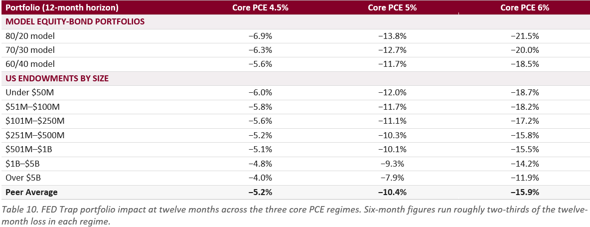
The regime gradient is close to linear in the inflation level but steepens between 5% and 6%, where credit widening more than doubles. Note that the 4.5% regime alone, which is well inside recent experience and requires no geopolitical trigger, already costs the peer-average endowment 5.2% over twelve months, before considering any of the oil tails.
5. Appendix: Portfolio Risk Detail and Methodology
5.1 Historical Stress Tests
Applying realized crisis episodes instantaneously to the same portfolios, using the actual factor covariance matrix and historical factor variations, makes the regime dependence explicit.
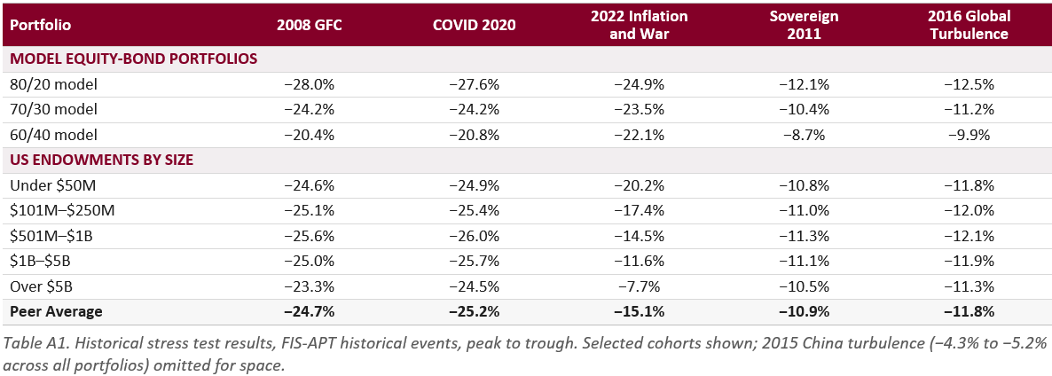
In a 2008 or COVID replay the endowments lose more than the 60/40, because the scenarios are growth shocks in which duration rallies and the balanced portfolio is protected. In 2022 the ordering inverts completely: the 60/40 loses 22.1% against 7.7% for the largest endowment cohort. All four forward-looking scenarios in this study are inflationary regimes like 2022, not growth shocks like 2008 which is why the size gradient runs the direction it does in Section 4.
5.2 Ex Ante Volatility, Factor Risk and Tail Measures
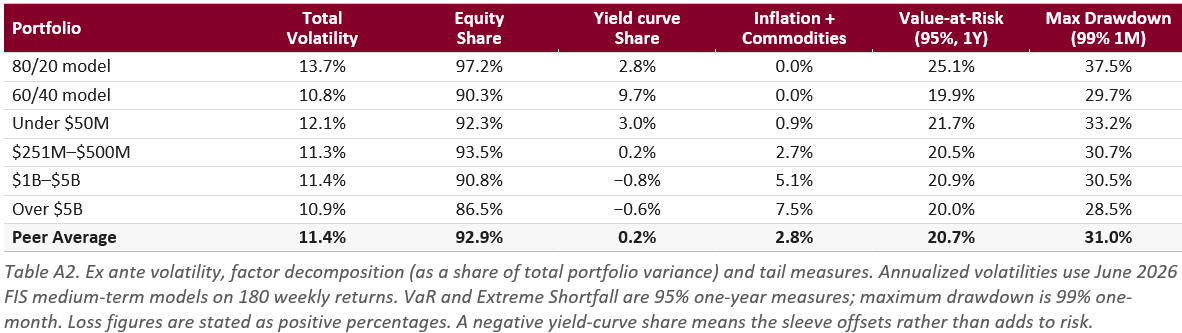
Total ex ante volatility barely separates the cohorts, running from 12.1% for the smallest to 10.9% for the largest, with the 60/40 lowest of all at 10.8%. Equity risk dominates every portfolio, explaining 86.5% to 93.5% of variance, which shows that even alternatives-heavy endowments carry meaningful equity beta. The difference sits in the non-equity exposures: model portfolios carry all of theirs in the yield curve (9.7% for the 60/40) while endowments carry almost none and instead pick up inflation and commodity risk that grows with size (from under 1% in the smallest cohort to 7.5% in the largest). This reflects the real assets allocation in Table 7 and is why the large cohorts hold up better in the oil-driven tails.
The gap between ex ante measures and scenario results is the central methodological point. One-year 95% VaR runs from 21.7% for the smallest cohort to 20.0% for the largest, a spread of under two points, while the FED Trap at twelve months separates the same two cohorts by nearly seven. Ex ante measures are calibrated on full-sample covariance and do not know that a shock is inflationary. That gap is the case for running scenario work alongside Value-at-Risk, not instead of it.
5.3 Methodology
The factor set follows the FIS global multi-asset class statistical factor model. Shocks are applied as additive percentage changes for prices and additive basis-point changes for yields and spreads, so a +70% oil shock and a +285 bps spread shock are both layered onto the 14 August baseline rather than absolute targets. The risk model covariance matrix is estimated using 180 weeks of equally weighted returns. The covariance structure used for the distance analysis comes from a backtest on monthly data from 2006 forward, with three-year windows for historical events. That window is deliberately long because it must contain enough genuine crises to serve as a fair yardstick covering 2008, the 2011 European debt scare, the 2015 China devaluation risk-off, the 2020 pandemic crash and the 2022 inflation shock. Collectively, these historical events provide the model a realistic sense of how far markets can move and how factors tend to move together.
This document does not constitute investment advice. Scenarios are modeled estimates designed to stress-test portfolio resilience under extreme but plausible geopolitical and macroeconomic conditions. Copyright © 2026 CISDM, Isenberg School of Management, University of Massachusetts Amherst. All rights reserved. FIS, APT and the FIS APT factor model are trademarks or registered trademarks of FIS or its subsidiaries.