By Masao Matsuda, CAIA, FRM, Founder, Crossgates Investment and Risk Management In January 2020, the CAIA New York Chapter organized an event titled “Volatility? Downside Protection? Asset Allocation & Factor Management Tools for the Coming Decade.”[i] In retrospect, the event was uncannily prescient, as just a few months into the new decade the market has seen extraordinary turbulence. Such market developments further reinforce the imperative to explore an important dimension of diversification in pursuing downside protection. Though not frequently addressed, a particularly important dimension of diversification is the relationship between time-varying equity volatility and the performance of major assets. Specifically, in those months with higher volatility equity securities on average tend to perform poorly compared to their performance in those months with lower volatility. To illustrate, using standard deviations of daily equity returns (NYSE, AMEX, and NASDAQ combined) for each month, one can examine the performance of equity returns by high or low volatility regimes. Those months with a higher standard deviation than the median value of standard deviations are classified as “high volatility months,” and those months with a lower standard deviation than the median value are considered “low volatility months.” Table 1 summarizes the results for the 70-year period from January 1949 to December 2018, as well as for seven 10-year periods. The table shows that the average monthly return in the high volatility months was 0.190% while that in the low volatility months was 1.762%. Astonishingly, the latter is more than 9 times higher than the former. Moreover, with both the high volatility regime and the low volatility regime having a sample size of 420 months each, the difference in the mean returns was statistically significant at the 1% confidence level. In addition, for each 10-year period, the average was higher for low volatility months without exception and in four out of seven periods statistically significant differences from the returns in the high volatility months were recorded. Also, the largest monthly loss was greater in the high volatility months for the 70-year period, as well as each 10-year period, again without exception. The table also shows three different measures of risk: standard deviation, 95% Value at Risk (95% VaR), and Conditional Value at Risk (CVaR). The 95% VaR is regarded as a suitable measure of downside risk, and CVaR as a coherent measure of tail risk. It is quite illuminating that in terms of all three risk measures equity was consistently less risky in the low volatility months (highlighted in brown). Thus, one can ascertain that investing in equity in the low volatility regime brings higher returns with lower standard deviations, downside risk, and tail risk. The only criterion that accords better performance to the high volatility regime is the top 15% monthly return. Unlike other return measures and the three risk measures, this measure is consistently better in the high volatility months (highlighted in blue). It is as though investors in the high volatility months are willing to pursue casino-type gains in exchange for lower average returns and higher risks. Consequently, it does not seem rational to invest in equity in the high volatility regime if one can predict which volatility regime the next month will bring. 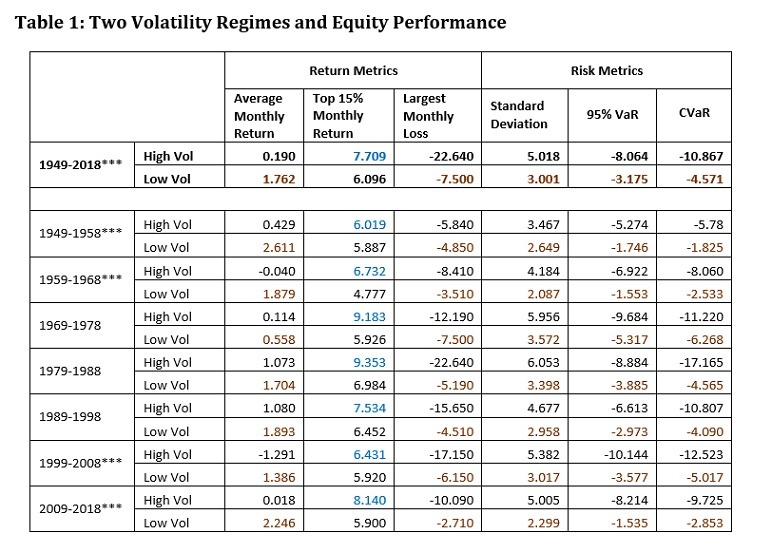 Note: When the low volatility regime performed better than the high volatility regime, it is highlighted in brown. Conversely, when the high volatility regime performed better, it is highlighted in blue. Data source is Kenneth French’s website covering equity securities in NYSE, AMEX, and NASDAQ. ***represents the period in which the difference in means of returns between the high volatility regime and the low volatility regime was statistically significant at the 1% confidence level. Equity volatility is known to persist, and a high volatility month is likely to be followed by another high volatility month. Let us explore the possibility of utilizing volatility forecasts for diversification purposes with an example of a simple 2-way allocation between equity and bonds for the 20-year period from January 1999 to December 2018. In the following analysis, we will use a 60-day Exponentially–Weighted Moving Average (EWMA) to forecast the next month’s volatility. In order to predict January 1999’s volatility regime, one needs to use volatility information prior to that month. For this purpose, the average of the forecast results from 1979 to 1998 (20 years) was compared to the volatility forecast for January 1999.[ii] If the average is higher than the expected volatility for a given month, that month is assigned to the low volatility regime, and one invests 100% of assets in US equity. Conversely, if the average is lower than the expected volatility, that month is assigned to the high volatility regime, and one invests 100% of assets in US government bonds. For a static asset allocation, decisions are simple — allocation weights to equity range from 0% to 100% with corresponding bond weights ranging from 100% to 0%.
 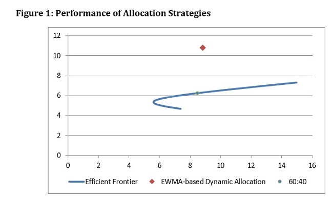 Note: Data sources are Kenneth French’s website covering equity securities in NYSE, AMEX, and NASDAQ and Swinkels, L. (2019) Data: International Government Bond Returns Since 1947, figshare. Dataset. Figure 1 shows the efficient frontier based on the monthly returns of US equity and government bonds during the 20-year period from 1999 to 2018. The frontier depicts static allocation with the equity weights ranging from 0% to 100%, while allocation is rebalanced to maintain predetermined weight. The blue point on the frontier represents the 60:40 allocation, a typical weight for many institutional investors’ strategic allocations. The red diamond indicates the 20-year average of the dynamic allocation based on the EWMA-based volatility forecasts. The dynamic asset allocation (DAA) unmistakably dominates the static allocation. If one were to maintain a certain strategic weight over the course of 20 years, one could not have done better than a point along the efficient frontier. Table 2 summarizes the result of the dynamic allocation and the 60:40 allocation. In terms of three return criteria, the DAA outperformed the 60:40. In terms of risk criteria, the only measure in which the 60:40 performed slightly better than the DAA was the standard deviation.
 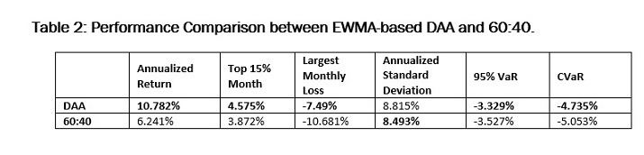 Albeit in the long run the DAA is shown to provide a better result, it may not always be the case for a given year. As a matter of fact, in the following five years out of the 20-year period, the 60:40 outperformed the DAA: 1999, 2003, 2009, 2012, and 2015. The last year, 2019, happens to be the year in which the simple 60:40 could have outperformed the DAA. For example, using an equity ETF (SPY) and a bond ETF (AGG) and extending the previous volatility forecasts beyond 2018, the DAA would have generated a 10.50% return for the year, while the 60:40 would have generated 22.33%. Not surprisingly, however, this situation has quickly reversed in 2020. The DAA would have avoided having exposure to equity in March and generated a loss of -2.662% for the first 3 months, while the 60:40 would have experienced a larger loss of -3.656%. The primary goal of diversification is to improve risk-reward ratios and to avoid downside and tail risks. In a static allocation, the benefit of diversification easily reaches its limit as the availability of asset classes with low correlation becomes limited or the underlying correlation structure among assets changes. It is evident that by explicitly focusing on time-varying volatility, one can further the goal of diversification with potentially higher returns and lower risks (standard deviations, downside risk and tail risk). At a time of major market turmoil, one critically needs a dimension of diversification that does not always presume to maintain exposure to the market risk. Pursuing allocation alphas can lead to better diversification and mitigation of downside and tail risks. [i] The moderator of the event (Jerome Abernathy) posed key questions such as “how can we use individual factors to mitigate risk in equity and bond portfolios?” The panelists, two portfolio managers (Graham Rennison and Amit Sinha), a consultant (Adam Duncan), and a risk manager (Michael Daly), in turn, provided their valuable insights. [ii] To be exact, the value of EWMA at the end of December 1999 becomes the forecast for January 1999. For this reason, the information starting in December 1978 to November 1998 was used. In subsequent months, the number of months utilized to calculate the average forecast result becomes larger by one month as each month goes by. Contact Masao Matsuda at matsuda@crossgates-im.com LinkedIn or Twitter @MasaoMatsuda