Did correlations among asset classes approach one during COVID-19 Crash? The short answer is no. Did the benefits of diversification disappear? The short answer is no, again.
During the last few weeks, several pundits have resurrected the old argument that, during increased market turbulence, diversification benefits disappear because correlations among investments approach one. I am here to cast doubts on both claims. Many of the same pundits use the same argument to question the benefits of passive investing. In those cases, one may want to question their motives. Back to our question:
Did diversification benefits disappear during the last month? No. In fact, those benefits increased. Since February 20 until March 12, we have seen the following index performance: RUSSELL Value (-28%), RUSSELL Growth (-22%), MSCI Ex-US (-24%), S&P 500 (-19%) and US Treasury 20+ (+8%). Certainly, a 60/40 portfolio would have experienced a much smaller drop. By the way, the Treasury index is up 15% since the beginning of the year. Further, the estimated correlation between Treasury and S&P 500 became more negative during this period. It changed from -35% during 2018-19 to almost -70%. Of course, as we see below, this estimated correlation is certainly wrong!
Did correlations approach one during the last month? No. This gets a bit technical. Some people confuse increased volatility with increased correlations. When they see increased volatility across various asset classes, they think correlations have increased. Their views are confirmed even more when they estimate the correlation and see that it has increased. To see how this works, perform the following simple simulation (it can easily be done using an Excel program).
- Create two standard normal random variables X and Y that have correlation 0.5.
- Sort the two variables based on the absolute values of X.
- Split the sample in two and calculate the correlations between X and Y using each subsample.
While the correlation between X and Y for the full sample is 0.5, you will notice that the correlation between X and Y for the subsample that consists of lowest absolute values of X will be around 0.22, and the correlation for the subsample that consists of the largest absolute values of X will be around 0.62! That is, calculating the correlation between X and Y when values of X are far away from the mean will give us an estimated correlation that is upwardly biased. By the same token, calculating the correlation when the values of X are close to the mean will give us an estimated correlation that is downwardly biased.
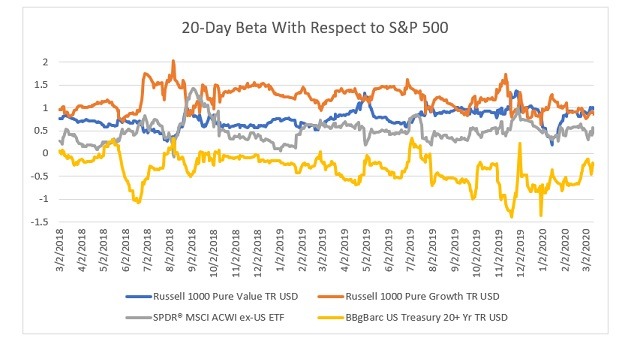
To see this, consider the definition of beta: Beta = Covariance(Y,X)/Variance(X), which measures the beta of Y with respect to X. It turns out that betas do not change much during increased market volatility (see the graph below and you can check it for the simulated data as well). If betas don’t change much, then the correlation estimated during periods of increased volatility will always be higher than the actual correlation even though the actual correlation has not changed at all. The higher the volatility, the higher our estimated correlation.
For example, the average correlation between the S&P 500 and MSCI Ex-US was 60% in 2018-19. Even if there is no change in the actual correlation, the increase in volatility (i.e., VIX) from about 13% to 70%, will give us an estimated correlation of 75%. Note that the actual correlation is still 60%. You may be surprised to know that the estimated correlation between the S&P 500 and MSCI Ex-US during the last month was indeed 75%!!! That is, the apparent increase in the estimated correlation is entirely due to increased volatility.
This calculation is based on the paper by Forbes and Rigobon (2000). There are some assumptions underlying their model that may not be satisfied in the real world. Still, their results are robust and, in some cases, the estimated correlation will increase even further if some of those assumptions are relaxed. There are other approaches to estimating correlation conditioned on changing volatility and they report increased correlation among asset classes during the GFC. Also, the above results do not apply to options or any security that has embedded options as the relationship will be nonlinear.
For those who are curious, the relationship between estimated correlation and actual correlation is this:
Estimate Correlation = Actual Correlation/Sqrt[(1+d)/(1+d*Actual Correlation)]
Here, d is the percentage increase in the volatility of the S&P 500.