


By Dan diBartolomeo, President and founder of Northfield Information Services, Inc. Based in Boston since 1986, Northfield develops quantitative models of financial markets.
One of the most basic assumptions of modern investment practice is that financial indices often used as benchmarks (or passive portfolios) are inherently well diversified. This assumption arises from several early research papers addressing “How many stocks does it take to make a diversified portfolio?” The answers varied widely from ten in Evans and Archer (1968) up to around forty Statman (1987). However, these papers all used a specific definition of what constitutes a “well diversified” portfolio in a single asset class context, “Is my portfolio sufficiently like the market so that idiosyncratic risks of specific assets are low?”
For most investors, the common understanding of the term “diversification” implies that sources of risk are largely independent across portfolio assets. This conception means that the returns from each financial portfolio asset should be uncorrelated with others within the portfolio. This “lack of correlation” is the motivation for many multi-asset class investors to seek low-correlation assets such as hedge funds and commodities.
Our two different conceptions of what diversification means are mathematically incompatible. Under the first definition, diversification is increased when idiosyncratic return behavior is low, while under the latter definition, diversification is increased when idiosyncratic return behavior is high. In the context of a multi-asset class portfolio, we may well ask if broad financial market diversification of passive indices is simply a myth?
Reconciling these two concepts of diversification brings forward two interesting conclusions. First, traditional “stock picker” equity portfolio managers should use quantitative methods to determine portfolio weights. The second is that the credit risk of many fixed-income portfolios may be significantly underestimated by popular analytical methods.
A historical perspective may be valuable to put the matter into context. In Shakespeare’s play The Merchant of Venice, the main character is asked if his business affairs are causing him to be worried. He replies with a very succinct representation of diversification.
Believe me, no: I thank my fortune for it.
My ventures are not in one bottom trusted,
Nor to one place, nor is my whole estate
Upon the fortune of this present year:
Therefore, my merchandise makes me not sad.
Readers who recall the play will remember that things didn’t work out too well for the Merchant in the end.
To resolve this confusion of meanings we will introduce a proprietary measure of diversification that captures the correlation among investment assets that is more appropriate in a multi-asset class setting. We believe this new measure is more aligned with what investors interpret the word “diversified” to mean. Our new measure is expressed as the number N (e.g., 20) of equally weighted positions that would be a comparably diversified portfolio, assuming each security had the average level of volatility of all members of the index, and all securities are uncorrelated.
Our empirical examples using equity market indices illustrate that due to capitalization weighting and correlation across securities, many popular indices that contain hundreds or even thousands of securities are far less diversified than investors presume. The disparity in understanding diversification in fixed-income portfolios is even more extreme.
The “Index of Diversification” is just
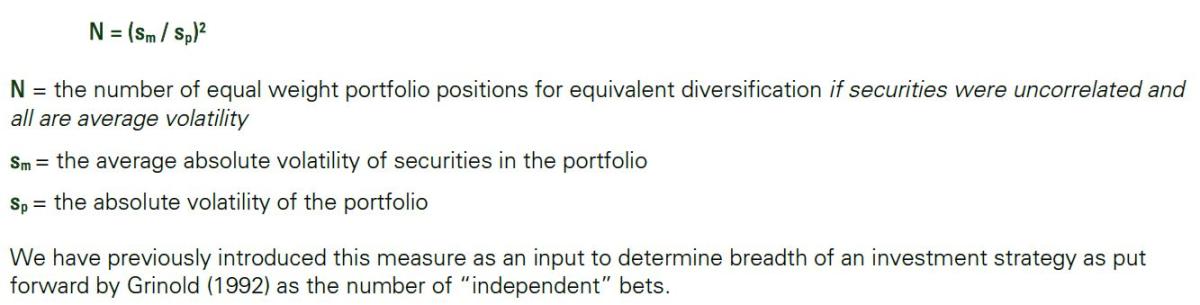
We have previously introduced this measure as an input to determine breadth of an investment strategy as put forward by Grinold (1992) as the number of “independent” bets.
Let’s do a quick example of the US top 1000 stocks using risk forecasts from the Northfield Fundamental model as of January 31, 1989. The forecast annual volatility of the capitalization-weighted US top 1000 is 19.01%, while the comparable metric for a portfolio of the same securities on an equal-weighted basis is 20.84%. At the same moment and using the same forecasting model, we get an average estimated volatility of 38.97% for the individual securities.
If all securities were of average volatility, equally-weighted, and uncorrelated, the forecast volatility of the equal-weighted portfolio would be just 1.23%, a small fraction of the 20.84% we have estimated with correlations across securities. Our index of diversification is just 4.20 suggesting that the degree of risk reduction arising from the capitalization-weighted portfolio is equivalent to just four portfolio assets of average risk and no correlation. We can conclude that the preponderance forecast risk is the result of covariance, suggesting a severe failure of diversification under our latter definition.
If we repeat our example at the more recent date of May 31, 2022, we get very similar results. The forecast volatility of the capitalization-weighted US top 1000 stocks portfolio is 20.99%, while we get 20.34% on an equally weighted basis. The average forecast volatility of the individual stocks is 40.80%. These values lead to a forecast volatility assuming zero correlation across the equal-weighted portfolio of 1.29%. Our index of diversification is 4.07, again illustrating an extreme failure of diversification under our second definition.
If we convert all the volatility values to return variances (volatility squared) the picture becomes even more transparent. The forecast variance of the capitalization-weighted portfolio is 440.58, while the forecast variance of the equal-weighted portfolio is 413.76. The average return variance of the individual securities is 1664.64. For the hypothetical case of a portfolio where every asset has the average volatility and correlations are zero, the forecast variance is 1.664. Again, the vast preponderance of risk is coming from the fact that the portfolio asset returns have covariance.
If we consider the situation of participants in international financial markets, we can see that there is a modest amount of improvement. We will operate with the Northfield global model as of May 31, 2022, with the top 1000 stocks that existed globally rather than being limited to those that traded in the United States. We assume the investor is based in US$. The forecast volatility of the capitalization-weighted global 1000 stock portfolio is 17.78%, while the forecast volatility of the equal-weighted global top 1000 stocks is 16.54%. The average forecast volatility of the individual stocks in the global 1000 is 39.80%. Our index of diversification is now 5.01, somewhat better than the 4.07 indicating the modest benefit of international diversification. The forecast volatility of the hypothetical portfolio of equally weighted, equal risk but uncorrelated assets is just 1.26%.
In variance terms the capitalization-weighted value is 316.13. The equal-weighted forecast variance is 273.57, while the average variance of the individual global stocks is 1558.04. Again, almost all the variance in portfolio returns arises from covariance rather than variance. It should be noted that for non-US international investors the picture is somewhat brighter. Many of the companies in our global top 1000 sample are based in the USA so there is no international diversification for that part of the portfolio for US-based investors. For an investor based in another country and currency, the portion of the global portfolio that would be effectively domestic would be far smaller.
We can further illustrate our assertions using the tool of mean/variance optimization as defined by Markowitz (1952, 1959).
Our goal is to create a “maximum diversification” portfolio as defined by Choueifaty and Cognard (2008) which is to minimize the magnitude of portfolio risk arising from covariance among the assets. We will use an optimization algorithm that allows us to minimize average correlation across securities by having levels of very low-risk tolerance to risks arising from common factors across assets and high tolerance to idiosyncratic risk.
Using the same model as of May 31, 2022, we obtain that the maximum diversification portfolio among the top 1000 US stocks had a forecast volatility of 15.81% (variance = 249.85) as compared to 20.99% (variance 440.58) for the capitalization-weighted portfolio. Of the portfolio variance, 57% arises from covariance as compared to 99.7% for the capitalization-weighed portfolio.
Most importantly, the maximum diversification portfolio under this definition contains just ten securities. Of the ten, eight are ADRs again illustrating the benefit of international diversification. For equity investment managers, such a result suggests that highly concentrated portfolios (e.g., ten assets) can be considered low-risk and well-diversified under definitions that are aligned with the beliefs of most investors. Such a result should give “stock picker” type managers new impetus to consider use of quantitative portfolio construction methods as first proposed in Bernstein and Tew (1994).
In terms of optimal portfolio construction, numerous papers such as Chopra and Ziemba (1993) have argued that estimation errors in returns dominate, with errors in volatility estimates of second importance and correlation in third place. Our results suggest that while individual pairwise correlations may not matter very much, estimation error in the average value of pairwise correlation greatly dominates estimation error in the volatility of individual securities.
This provides strong evidence that factor models will always provide better portfolio-level risk estimates as compared to historical observation as factor models effectively filter out past events that are unlikely to be repeated. For example, the two stocks of otherwise unrelated companies might both drop on the same day if both their respective CEOs were killed in the same airplane crash. As the likelihood of such an event happening again is almost nil, our expectations for future correlation of returns should largely ignore the effect of this incident. For more discussion of factor models see diBartolomeo (2014).
Various methods can be employed to calculate the expected average pairwise correlation across the members of a portfolio or index. Every security covariance matrix whether historical or forecast can be approximated by a factor model, inclusive of the filtering effect. Since an equal sign works in both directions, this implies that any factor model output can be converted back to the numerically equivalent full covariance matrix.
Once we have the equivalent full covariance matrix, we can divide through by the relevant volatilities to give the implied asset correlation matrix. We can obviously take the average of the off-diagonal elements of the correlation matrix. The algebraic details are provided in See diBartolomeo (1998) Optimization with Composite Assets Using Implied Covariance Matrices (northinfo.com). For simple one factor models (e.g. CAPM) the algebra is trivial. An alternative method for estimating average asset correlation based on observing cross-sectional dispersion of security returns is provided in Solnik and Roulet (2000).
An important implication of our results is that investors are likely to be underestimating “tail” (extreme return event) risk for benchmarks and passive index portfolios. It is widely assumed in financial models that asset returns are normally distributed, but individual security returns have “fat tails” (e.g. T-5), particularly when observed over shorter time horizons (e.g. daily). A full discussion appears in diBartolomeo (2007, Professional Investor) and Fat Tails, Liquidity Limits and IID Assumptions (northinfo.com).
The Central Limit Theorem requires that if we have enough independent distributions, the sum of those distributions will be a normal distribution. The T distribution becomes indistinguishable from normal for N > 40. Our result suggests that even for broad equity indices, the high average correlation means that the number of independent security return distributions is small (e.g. 5) so we should be evaluating tail risk for equity indices using a T distribution, not an assumption of normality.
Our analysis of equities also has important implications for analysis of credit risk for loans, corporate bonds, and even sovereign debt. Merton (1974) demonstrates that corporate debt can be replicated by a two-asset portfolio consisting of a riskless bond and an amount of equity in the borrower. Belev and diBartolomeo (2019) provide a parallel model linking the creditworthiness of sovereign bonds to the equity market of the country. To the extent that an individual bond almost always has more potential to fall in value (default) than rise, the distribution of returns will usually have negative skew and positive excess kurtosis. The presence of higher moments means that correlations across individual securities are even more impactful in terms of whether portfolio credit risk is as diversified as the investor may believe. If real-world fixed income portfolios are not sufficiently diversified, then credit risk assessment measures that assume symmetric distributions (e.g. “duration times spread”) are inappropriate.
The assumption that equity indices are “well diversified” is highly suspect. If we define diversified to mean “like the overall market” any broad equity index will be obviously like itself. However, if investors understand well diversified to mean that return risks arise from uncorrelated causes and events, then the level of diversification provided by equity indices is no better than a handful of individual stocks specifically chosen to have low correlation.
This concept is easily represented by defining a diversification index in terms of an equivalent number of equal weighted, equal risk, uncorrelated positions. The “number of equivalent positions” measure can be usefully employed in various ways including describing diversification and the “breadth” of active strategies.
All posts are the opinion of the contributing author. As such, they should not be construed as investment advice, nor do the opinions expressed necessarily reflect the views of CAIA Association or the author’s employer.
About the Author:
Dan diBartolomeo is President and founder of Northfield Information Services, Inc. Based in Boston since 1986, Northfield develops quantitative models of financial markets. The firm’s clients include more than one hundred financial institutions in a dozen countries.

Dan serves on the Board of Directors of the Chicago Quantitative Alliance and is an active member of the Financial Management Association, (“QWAFAFEW”), the Society of Quantitative Analysts. Mr. diBartolomeo is a Director of the American Computer Foundation, a former member of the Board of Directors of The Boston Computer Society, and formerly served on the industry liaison committee of the Department of Statistics and Actuarial Sciences at New Jersey Institute of Technology.
Dan is a Trustee of Woodbury College, Montpelier, VT, and continues his several years of service as a judge in the Moscowitz Prize competition, given for excellence in academic research on socially responsible investing. He has published extensively on SRI, including a forthcoming book (with Jarrod Wilcox and Jeffrey Horvitz) on portfolio management for high-net-worth individuals.