By Masao Matsuda, CAIA, FRM, Founder, Crossgates Investment and Risk Management One would think hedge funds can weather market gyrations better than long-only equity investments as hedge funds have greater flexibility in determining the levels of market exposure. However, while some individual hedge funds may have been successful in adverse market situations, an analysis of various hedge fund strategies at the index level reveals that they face challenges in navigating market turbulence. One reason can be found in hedge funds’ sensitivity to the time varying volatility of equity securities. This post analyzes the degree of influences time-varying volatility has on the performances of hedge fund strategies, and suggests a way to improve risk-reward ratios for hedge fund investments and seek further diversification benefits, using a dynamic allocation method based on predicted volatilities. Returns versus Three Types of Risk Figure 1 visualizes the performance differences of Eurekahedge hedge fund strategies between the high and low volatility equity regimes from January 2000 to March 2020. As was done in an earlier post, the sample (243 months) is divided into the two regimes based on the median monthly volatility for the period. 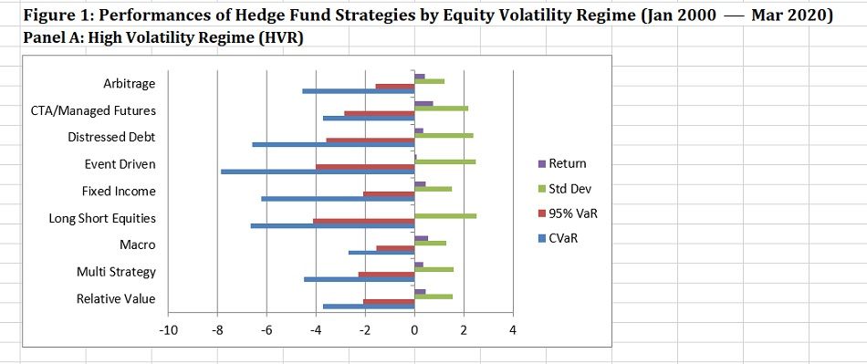
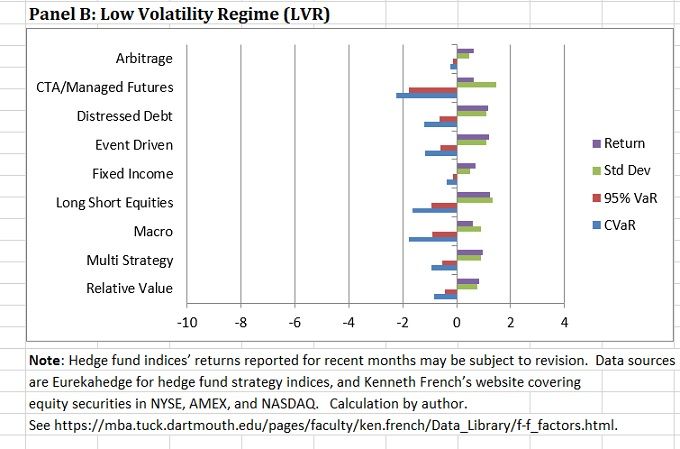 Shown to the right of the “zero percent” axis are the average monthly returns and the standard deviations of nine hedge fund strategies. To the left are the 95% Value at Risk (95% VaR) and the Conditional VaR (CVaR) of each strategy.[i] In other words, the figure contrasts the “average monthly return” to three metrics of risk, i.e., standard deviation, downside risk (95% VaR) and tail risk (CVaR). Panel A shows the statistics for the high volatility regime (HVR) and Panel B for the low volatility regime (LVR). Several important characteristics readily can be observed. First, the average return is higher in the LVR for most strategies, sometimes at astonishing multiples. For instance, the Event Driven strategy’s return in the LVR (1.19%) is approximately 12 times higher than that in the HVR (0.10%), and the Long Short Equities strategy’s return in the LVR (1.22%) is over 300 times higher than that in the HVR (0.004%). An exception is the CTA/Managed Futures strategy, which performed somewhat better in the HVR (0.75% vs. 0.63%). Second, the standard deviations are without exception higher in the HVR. The multiples range from 1.67 (Multi Strategy) to 3.5 (CTA/Managed Futures). On average, the multiples are 2.13 times higher. At a minimum, this indicates that equity market volatility strongly affects the volatility of each hedge fund strategy. Third, downside risk, as measured by the 95% VaR, is far higher in the HVR. The VaR figures range from -1.56% (Macro) to -4.14% (Long Short Equities) in the HVR, and they range from -0.12% (Arbitrage) to -1.78% (CTA/Managed Futures) in the LVR. In the case of the Fixed Income strategy, the multiple is around 16. On average, the VaR is 6.21 times higher in the HVR than in the LVR. Fourth, the CVaRs range from -2.68% (Macro) to -7.87% (Event Driven) in the HVR, whereas in the LVR they range from -0.24% (Arbitrage) to -2.23% (CTA/Managed Futures). The Arbitrage strategy has the highest multiple at around 19 as its CVaR for the low volatility is very small, even though its value in the HVR is moderate (-4.54%). On average, the CVaR is 6.77 times higher in the HVR. Taken together, it seems imprudent to invest in most hedge fund strategies in the HVR, as these strategies tend to deliver much lower returns with considerably higher risks. To make matters worse, the problem does not end with poor risk-reward ratios, as will be discussed below. Differences in Correlation Structure between Volatility Regimes
  Note: Figures in red indicate lower correlations in the HVR than in the LVR. Figures in brackets are correlation coefficients for the sample period (Jan 2000 – Mar 2020). Source: Eurekahedge and Yahoo Finance. Calculation by author. Table 1 shows the differences in correlation for a pair of hedge fund strategies between the HVR and the LVR. A positive (negative) number indicates that a pair has a higher (lower) correlation in the HVR. With the exception of the pairs involving CTA/Managed Futures and Macro strategies, correlations are invariably higher in the HVR, further diminishing diversification potential. The figures in brackets are the correlation coefficients for the sample period before the observations are divided into the two regimes. Out of 36 pairs, 28 pairs of hedge fund strategies have a correlation higher than 0.5. Moreover, 22 pairs have a correlation higher than 0.7. These observations signify the difficulty in seeking diversification among most hedge fund strategies when investments are maintained throughout the period, and worse yet when invested in the HVR. On the other hand, the CTA/Managed Futures strategy has low correlations with other strategies except with the Macro strategy. In addition, the correlations are lower in the HVR, resulting in the negative differences shown in the table. Take the case of correlation between the CTA/Managed Futures and Long Short Equities: in the HVR the correlation is 0.043 (not shown) and in the LVR 0.476 (not shown), resulting in a difference of -0.433. The other three pairs that exhibit lower correlations in the HVR involve the Macro strategy, though the differences are not large. The CTA/Managed Futures and Macro strategies are often viewed as potential diversifiers at a time of high market volatility. One needs to devise an allocation strategy which can maximize diversification benefits. Dynamic Allocation Based on Predicted Volatility One can take advantage of volatility forecasts to pursue dynamic allocation among hedge fund strategies. There are many time-series techniques to forecast volatility. In the analysis below, let us employ a simple Exponentially-Weighted Moving Average (EWMA) technique to forecast the volatility for the next month, using the past 60 days of daily data. One also needs a threshold level of volatility to determine the volatility regime to which each month’s forecast is assigned. For January 2000’s forecast, the average of the 20-year period of monthly forecasts ending in November 1999 is used as the threshold and is compared to the result calculated as of the end of December 1999, which becomes the forecast for January 2000. For subsequent months, the number of months to calculate the threshold level of volatility increases by “one” each month. If the forecast is lower (higher) than the threshold volatility for a particular month, it is assigned to the low (high) volatility regime.[ii] As discussed previously, some hedge fund strategies performed well in the LVR, and others did well in the HVR. For the purpose of dynamic allocation among hedge fund strategies, let us choose three strategies with the highest returns for each regime. This means that for the LVR, Distressed Debt, Event-Driven, and Long Short Equities strategies are chosen. For the HVR, the CTA/Managed Futures, Macro, and Relative Value strategies are chosen. These strategies are equally-weighted within each regime. To evaluate the effectiveness of dynamic allocation, a benchmark portfolio is created with an equal weight given to each month for each of the six strategies included in the two regimes.
 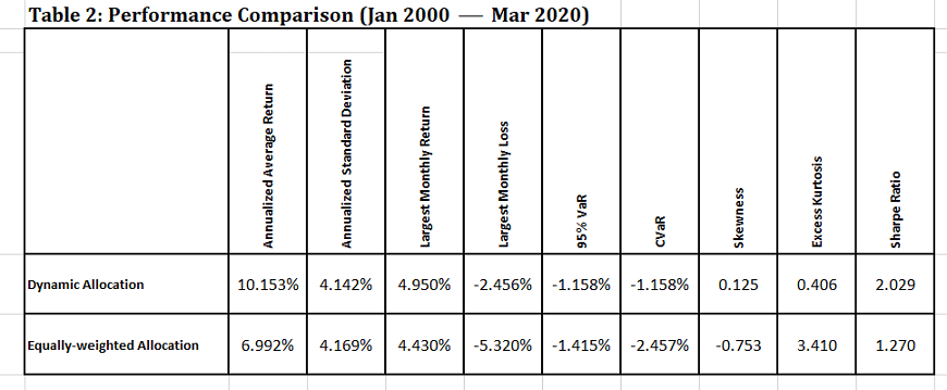 Table 2 compares the results of the dynamic allocation strategy to those of the equally-weighted allocation strategy in the January 2000 to March 2020 period. The dynamic allocation’s annualized average return is much higher than that of the equally-weighed allocation, with a very similar level of standard deviation. This results in a much higher Sharpe ratio for the former. The dynamic allocation’s largest monthly loss is less than half that of the equally-weighted allocation, while the largest monthly return is larger for the dynamic allocation. The results for the dynamic allocation show that downside risk (95% VaR) is smaller than that associated with the equally-weighted strategy and tail risk (CVaR) is less than half that of the equally-weighted strategy. In addition, as a result of the dynamic allocation being based on time-varying volatility, the shape of return distribution becomes very close to normal with skewness of 0.125 and excess kurtosis of 0.406. In sum, for every criterion shown in the table, the dynamic allocation dominates the equally-weighted allocation. Implementing Dynamic Hedge Fund Allocation The Eurekahedge hedge fund indices are not investable indices. Therefore, the dynamic allocation demonstrated above cannot be directly implemented. However, there are liquid alternatives such as ETFs that mimic various hedge fund strategies, and transaction costs for these instruments can be extremely small. One should also take advantage of more advanced volatility forecast techniques to assign a correct volatility regime for each month with greater accuracy than the simple 60-day EWMA employed in this analysis for illustration purposes. [i] VaR and CVaR are often shown in absolute value terms. However, since these numbers are all in negative territory in this analysis, they are shown to the left of the 0% axis. [ii] There are 117 months belonging to the high volatility regime, and 126 months belonging to the low volatility regime. Contact Masao Matsuda at matsuda@crossgates-im.com LinkedIn or Twitter @MasaoMatsuda