

By Daniela Hanicova, Quant Analyst and Product Developer at Quantpedia.
High Inflation Periods
Inflation is a measure of an increase in prices over time. Most typically, we measure inflation on a yearly basis. We say that inflation is high when the annual increase in prices of goods and services is unexpectedly increased. You might ask what triggers these periods. Most typically, geopolitical conflicts.
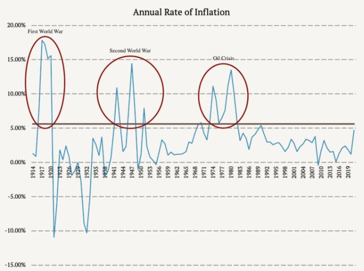
In this article, we analyzed the Consumer Price Index from the Federal Reserve Bank of Minneapolis, which includes the rate of inflation in the USA since 1913. Firstly, we calculated the top quintile and looked at which years inflation was higher. Therefore, we consider years with inflation above 5.62% high-inflation years.
Accordingly, there have been several high inflation periods since 1913. More specifically, we identified three clusters: 1916 – 1920 (First World War), 1942 – 1951 (Second World War), 1970 – 1982 (1973 Oil Crisis). And as the figure shows, another high inflation period might be coming soon.
First World War
As previously mentioned, geopolitical conflicts tend to trigger high inflation, and the first world war was not an exception. The annual rate of inflation before and at the beginning of the 1WW was around 1%. However, it rose to 7.7% in 1916 and 17.8% in 1917. The inflation rate stayed abnormally high until 1920 and fell to deflation (-10.9%) in 1921. Unfortunately, we do not have factor performance data from this period, so this period is excluded from further analysis.
Second World War
As you might have expected, the following high inflation period occurred during and after the second world war. The annual inflation rate started to grow in 1941 and reached 10.9% in 1942. As the war ended in 1945, inflation was unexpectedly low. However, it rose again in 1946 to 14.4%. The rapid post-war inflationary episode was caused by the elimination of price controls, supply shortages, and pent-up demand. Additionally, in 1951, the Korean war started. Overall, the average inflation between 1942 and 1951 was 5.94%.
Oil Crisis of 1973
The last high inflation period we analyze is the period around the 1973 oil crisis. The crisis was a direct consequence of the Arab-Israeli War. Arab members of OPEC (the Organization of Petroleum Exporting Countries) restricted the U.S. because of their relationship with Israel. The U.S. was re-supplying the Israeli military to gain leverage during the post-war peace negotiations. The inflation rate rose from 3.3% in 1972 to 6.2% in 1973 and 11.1% in 1974. It stayed abnormal until 1983 when it fell to 3.2%. But high inflation in this period can’t be just blamed on the geopolitical situation; some steps of the FED were probably also the source of the inflation problem.
High Inflation Periods Analysis
The second world war and the 1973 oil crisis are the main subjects of this article. We analyze the Fama and French 3 Factors (Mkt, SMB, HML), Momentum, Short-Term Reversal Factor, Long-Term Reversal Factor, and 10 Industry Portfolios during the time of the events. We exclude the first world war, as we do not have data for this period.
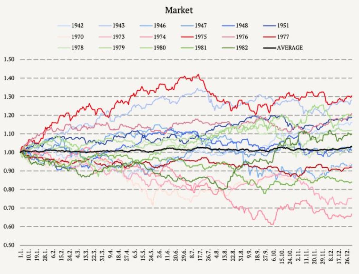
The figures in this section follow a color scheme:
- 1942 – 1951: light blue to dark blue
- 1970 – 1977: light red to dark red
- 1978 – 1982: light green to dark green
so that it is easier to recognize individual years.
Market During High Inflation Periods
Firstly, we analyze the market’s movement during the abovementioned one-year periods. The following figure illustrates the equity curves of the market. The black curve represents the market’s average performance during the individual years. On average, the yearly performance of the market portfolio is 3.28%. While the average market performance is not small, it is definitely smaller than in the years when the inflation is not so high. The distribution of yearly returns is nearly symmetrical, but it seems that the 1970s were worse than the 40s or 80s.
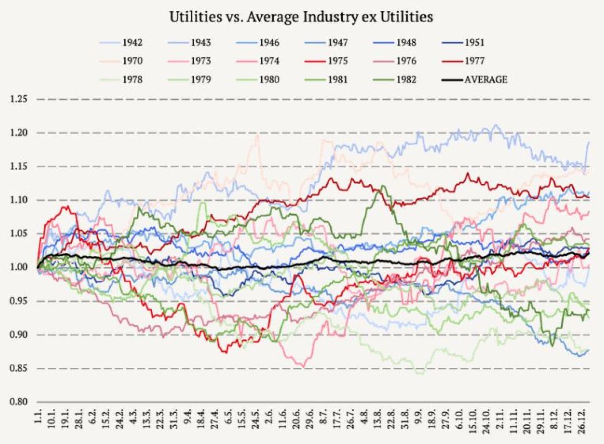
Safe-Haven Assets During High Inflation Years
Secondly, we look into how safe-haven assets would behave during the years of high inflation. We use the 10 Industry Portfolios to create a bond-like portfolio by going long utilities and shorting the average of the nine industries ex. utilities. The long-short portfolio should have a bond-like payoff. On average, the yearly performance of such safe-haven portfolio is 2.07%. Here, the pattern is clear, the worst performance was in the late 70s and the beginning of the 80s when the inflation shot up, and the FED started to increase short-term interest rates to over 10%.
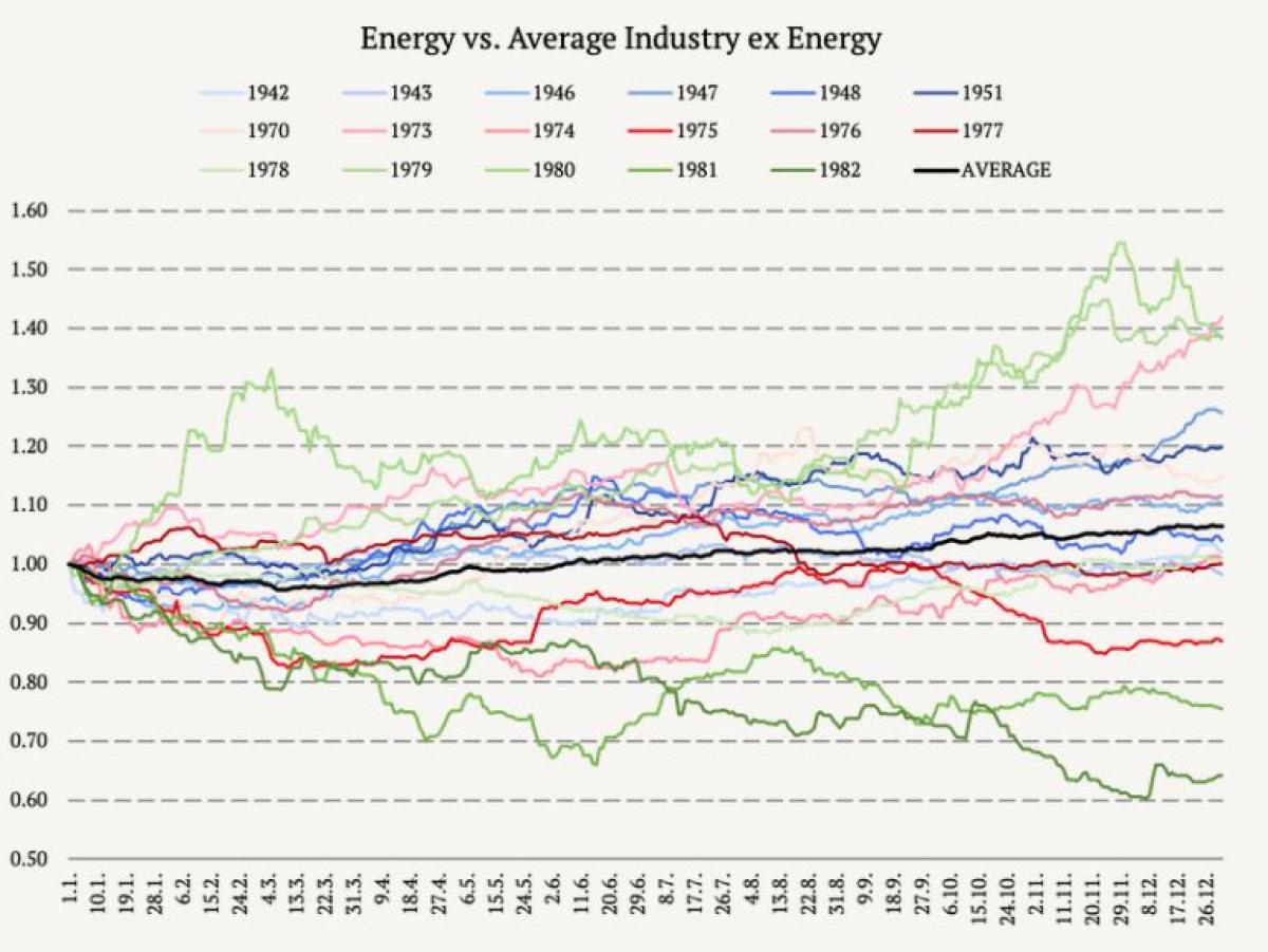
Energy Prices Proxy
Additionally, we examined the energy prices proxy/ crude oil proxy by calculating another long-short portfolio. Again, we analyze the 10 Industry Portfolios, and we calculate a portfolio that goes long energy and shorts the average of the nine industries ex. energy. On average, the annual performance of the energy price proxy is 6.37%. It’s not unexpected; the energy stocks are a natural hedge for the period of high inflation. The performance was nearly always positive; the only really bad years for energy stocks were 1981 and 1982, the years at the end of the 1970s and 1990s high inflation cycle.
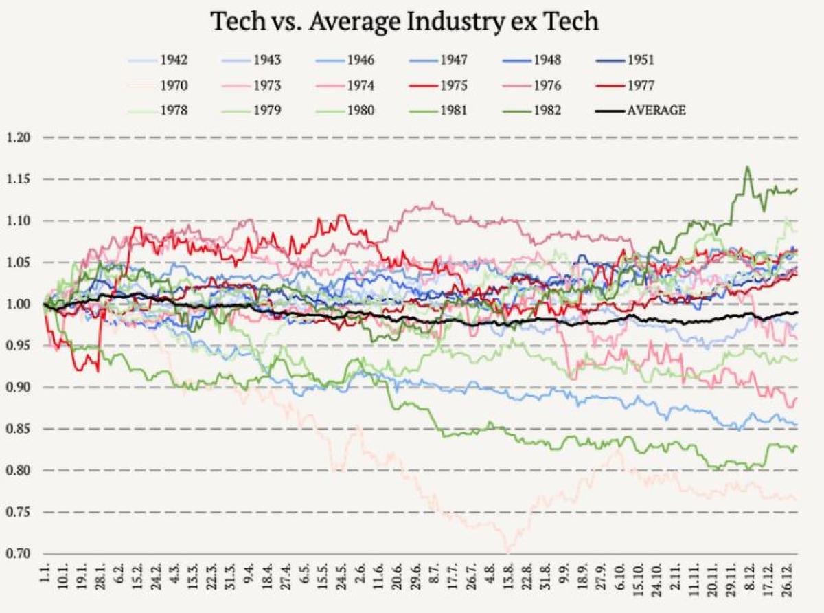
Tech Portfolios During High Inflation Years
Furthermore, we examined the tech prices proxy by calculating another long-short portfolio. Again, we analyze the 10 Industry Portfolios, and we calculate a portfolio that goes long tech and shorts the average of the nine industries ex. tech. Overall, the tech industry performs the worse during the high inflation periods. On average, the annual performance of the tech price proxy is -1.01%. This finding is probably the most important of our analysis. The tech sector is usually hit more than the sector of utilities; that is probably caused by shrinking the P/E ratios for high growth stocks. Tech stocks have usually higher implied duration, which causes their underperformance as rising inflation and rising rates are constantly re-pricing the future value of tech stocks.
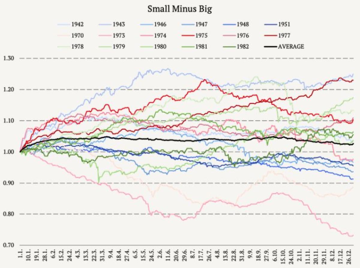
SMB and HML
Small Minus Big (SMB) and High Minus Low (HML) are two of the Fama and French 3 Factors. SMB is defined as the average return on the three small portfolios minus the average return on the three big portfolios. The average annual performance of the SMB factor is 2.68%.
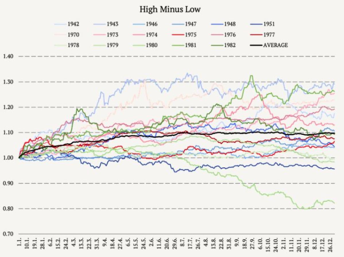
Secondly, HML is defined as the average return on the two value portfolios minus the average return on the two growth portfolios. The average annual performance of the HML factor is 9.68%. Now, compare this to the bleak performance of the tech stocks. It seems that value stocks (together with energy stocks) are the natural leaders for periods of high inflation.
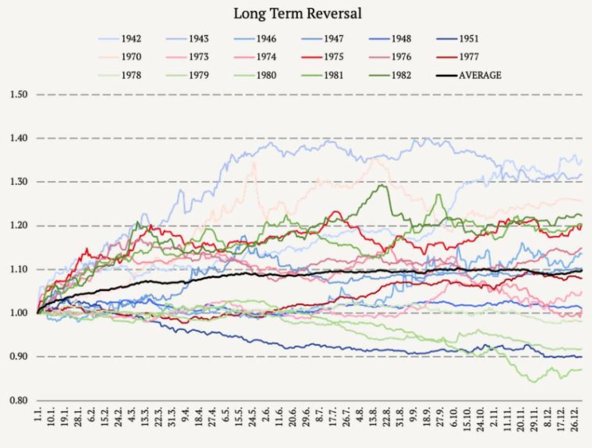
Long Term Reversal Factor
In this section, we explore the long-term reversal factor. The performance of long-term reversal was mostly positive during the majority of the high inflation years. The only exceptions were 1951, 1979, and 1980, where the performance declined. On average, the yearly performance of the long-term reversal factor is 9.75%. The long-term reversal effect is vaguely similar to Fama& French HML factor, but it doesn’t use the balance sheet information, just the information from stocks’ prices alone. Our analysis also shows attractive performance in high inflation periods.
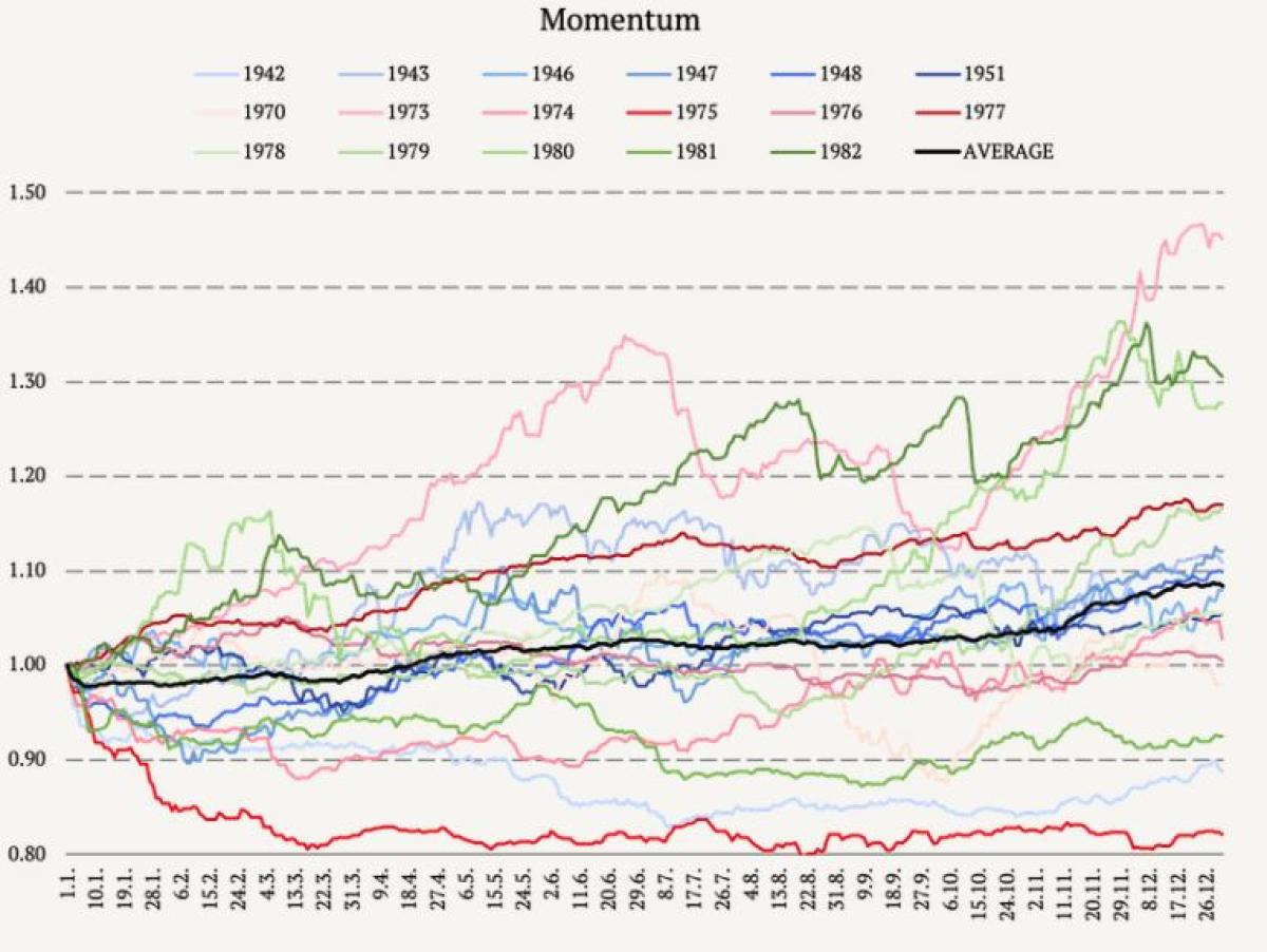
Momentum Effect During High Inflation Periods
Unlike the long-term reversal factor, the performances of the momentum effect are more unevenly distributed. During most years, the performance of the momentum factor is around 0%. However, there are a few years with an abnormal yearly return, specifically 1973, 1980, and 1982. And a few with significantly bad performance: 1942, 1975, 1981. On average, the annual performance of the momentum factor reaches 8.43%.
Conclusion
This article examines high inflation periods. We defined high inflation as above 5.62%, which is the top quintile, calculated from the data from 1913 to 2021. We found multiple years during which the inflation was abnormally high. As the high inflation periods cluster, we defined three periods: 1916 – 1920 (First World War), 1942 – 1951 (Second World War), and 1970 – 1982 (1973 Oil Crisis).
We analyzed the Fama and French 3 Factors (Mkt, SMB, HML), Momentum, Long-Term Reversal Factor, and 10 Industry Portfolios during the above-mentioned periods, excluding the first world war, as we do not have factor’s performance data from this period.
The article presents the performance of each factor during high inflation years. Also, average performance is calculated for each factor. Overall, the market factor’s average performance is 3.28%. The factors with the highest average performance are HML (value stocks), long-term reversal, momentum and energy stocks. On the other hand, tech stocks, bond-like assets and the SMB factor should be avoided during the high inflation periods.
However, all graphs show a large variance between the performance of individual factors over the years. Even though the average yearly return is higher/lower compared to the market’s return, the performance during individual years can vary significantly.
Another period of sustained high inflation is probably right around the corner, as the Russia-Ukraine Conflict keeps evolving, and its end is nowhere to be seen. So it would probably be wise to prepare for it.
About the Author:
Daniela Hanicova is a graduate of Comenius University, Bratislava, Slovak Republic, with a Master's degree in Probability and Statistics. Currently working at Quantpedia as Quant Analyst and Product Developer.

Great collaborator with excellent time management skills and analytical thinking who keeps deadlines and commitments.