


By Oliver Whitehead, Head of Investment Risk, and John Townhill, Quant on the Investment Risk team at Man AHL.
Looking for a powerful tool to identify return skewness and asymmetry, correlation breakdowns and heavy-tailed returns? Tail betas may be the answer.
Introduction
On 26 November 2021, news headlines were dominated by a new Covid-19 strain – Omicron – that was spreading rapidly in parts of South Africa. The World Health Organisation labeled it a “variant of concern” and the US, EU and other major destinations responded by blocking flights from several African countries.
In financial markets, news about the Omicron variant was met with a significant risk-off move across asset classes: the CBOE Volatility Index (‘VIX’) spiked by 10 points, among the five biggest single-day volatility moves in the past three decades1; the US 10-year Treasury yields decreased by 16 basis points, and equities and commodities sold off. Indeed, the moves in commodities were especially significant: WTI crude, for example, declined by 13.1%, an 8-standard deviation (‘SD’) move. To put this in perspective, an 8-SD decrease in WTI Crude has only happened twice since 19962.
Large moves in one asset class are often accompanied by large moves in other asset classes regardless of the recent correlations in markets.
The moves in each asset class were large compared with prevailing volatilities at the time. However, what was most striking about the moves on the 26th of November was the co-movement across instruments and asset classes. Figure 1 shows the hypothetical returns of a momentum strategy on that day (illustrated by the red cross) across different asset classes, compared with the possible outcomes simulated by Man Group’s internal risk model. The combined returns of stocks and currencies, and between stocks and bonds, were both on the very edge of possibility according to the risk model, illustrating the unlikeliness of the moves seen on 26 November given the recent market environment upon which the model is calibrated.
Figure 1. Hypothetical Returns of a Momentum Strategy Versus Outcomes Predicted by Risk Model
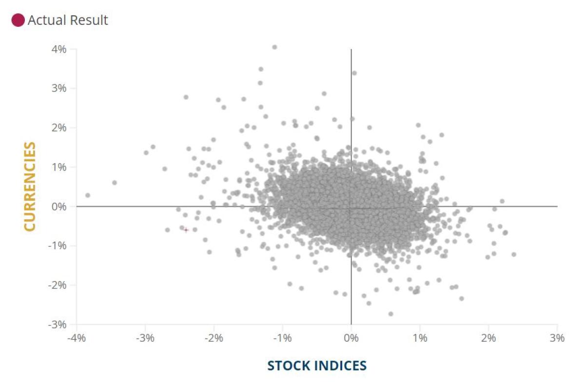
Source: Man AHL; as of 26 November 2021. Please see the important information linked at the end of this document for additional information on hypothetical results.
So, how should investors interpret risk measures during extreme moves where the correlation structure between assets may break down?
The Shortcomings of ‘Standard’ Betas During Extreme Market Moves
We’ve written before about betas and how to calculate the ex-ante beta of a portfolio to a factor3. To briefly recap: an ex-ante beta is the sensitivity of the current portfolio to a factor. A beta to a 1-SD move in a factor (the price of WTI Crude, for example) estimates the correlated impact on a portfolio’s P&L if crude oil prices were to increase by 1 SD.
Betas only consider typical moves in factors. As a result, they don’t allow for a breakdown in the correlation structure that could happen with large moves.
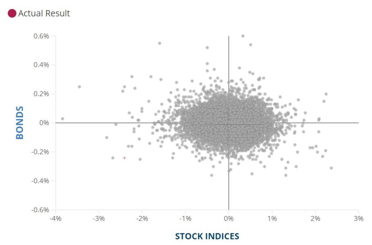
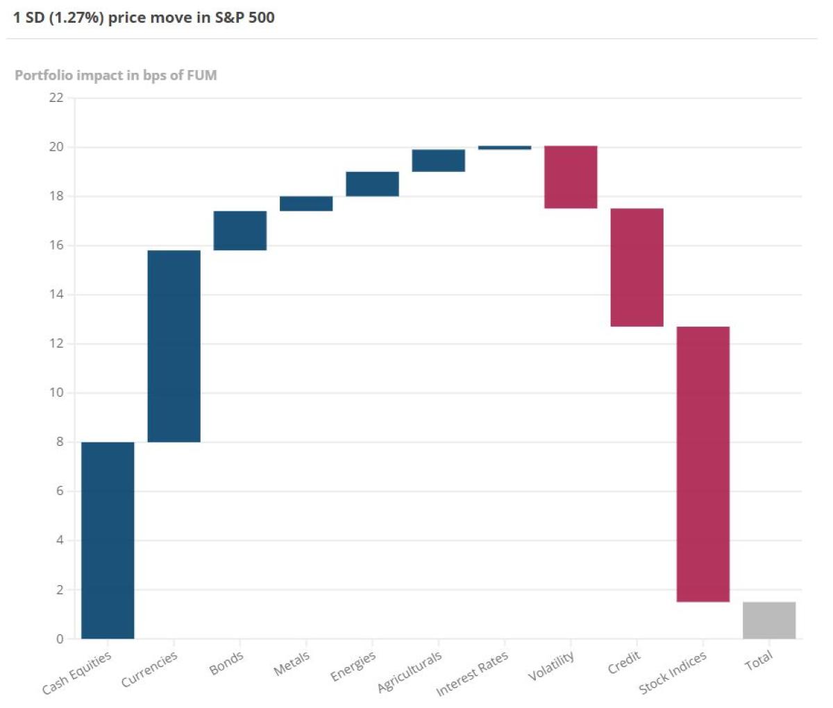
One of the attractive properties of beta as a risk measure is that it is additive. If we split our portfolio into sub-portfolios (for example, by asset class) and calculate the beta of each to crude oil, we can calculate the beta of the total portfolio to crude by summing up the sub-portfolio betas. We can visualize this decomposition per asset class to decompose the impact of the move in the factor into each sub-portfolio (Figure 2).
Figure 2. The Impact of a 1-SD Move in Crude on the Different Asset Classes in a Portfolio
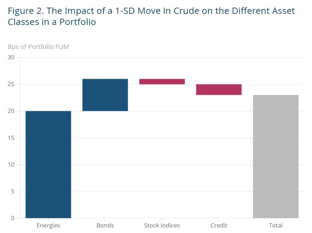
Source: Man AHL. For illustrative purposes only. Please see the important information linked at the end of this document for additional information on hypothetical results.
Ex-ante betas are a useful part of a portfolio manager or risk manager’s toolkit. However, calculating a beta typically makes use of a covariance matrix, which only describes a ‘typical’ dependence structure between assets, rather than their co-movement in a period of market stress.
For example, if bond-equity correlations were negative over the period a covariance matrix is calculated, deriving a beta will not capture the possibility of this correlation flipping to positive in a bond-driven equity selloff. Heavy tails which are empirically observed in asset returns will also not be captured during benign market periods.
The consequence of this is that a beta can often fail to capture the sensitivity of a portfolio to a sudden period of market stress and a corresponding shift in the risk properties of a diversified portfolio of assets, as seen on 26 November 2021.
A standard beta also doesn’t tell us anything about the asymmetry or heavy tails of financial asset returns. For example, the probability of a large down move in the S&P 500 Index is larger than the probability of a large up move, and large moves in either direction are more likely than using a normal distribution bell curve would imply.
A tail beta to a factor is the expected return of a portfolio under a tail move in that factor.
Introducing Tail Betas
In the same way that the standard beta of a portfolio is the expected P&L when a factor moves a ‘typical’ amount, a tail beta is the expected P&L when a factor moves by an extreme amount. More precisely, a tail beta is the expected value of the portfolio’s P&L conditional on a particular factor having an abnormally high (top 1%) or low (bottom 1%) return.
Note that the definition of tail beta is very similar to that of the commonly used expected shortfall (‘ES’) or conditional Value at Risk (‘CVaR’) risk measure, which is the expected value of the portfolio’s P&L conditional upon the portfolio P&L having an extremely low, say, bottom 1%, return.
The reason for using 1% as our definition of the tail is that it strikes a reasonable balance between being extreme, stable, and familiar:
- It would be inappropriate to consider events that happen more frequently than 1-in-100 days to be in the tail of the return profile;
- Using a tail size less than 1% could give unstable results due to a small sample size;
- Value at risk and expected shortfall are commonly calculated at the 99th percentile. As such, risk management teams should have already calibrated and back-tested their risk models at this part of the distribution.
An attractive property of defining the tail beta explicitly as an expected value is that – just like the usual tail betas – it is additive across sub-portfolios.
Calculating a Tail Beta
There are three steps in calculating tail betas:
- Simulate factor and portfolio returns;
- Filter the results conditional on the tail returns of the chosen factor;
- Take the mean.
This is best explained with a hypothetical example. Assume we want to calculate a tail beta of a bond-equity portfolio to a move in WTI Crude. To keep the example simple, we’ll use only 10 simulated days of data, and 20% as our definition of ‘tail’ (rather than 1%).
First, we perform our 10 simulations of our factor and portfolio returns. These could either be: (1) historical simulations, where 10 historical days of market moves are applied to the portfolio; or (2) Monte Carlo simulations, where assumptions about the distributions of each asset’s return and the dependency structure between them are made.
An example set of simulation results is shown in Figure 3.
Figure 3. Simulated Portfolio Returns Driven by Changes in WTI Crude
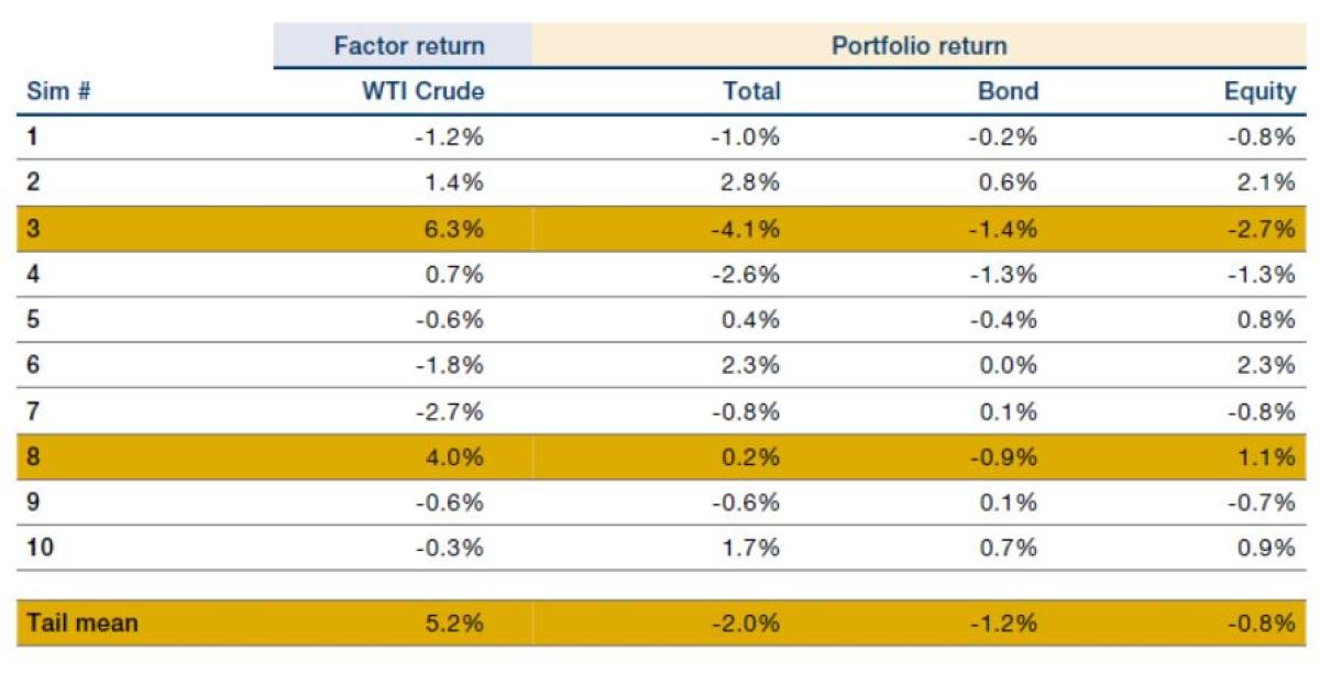
Source: Man AHL. For illustrative purposes only. Please see the important information linked at the end of this document for additional information on hypothetical results.
The next step is to filter the results on the factor tail, i.e., to look at the 20% of simulations with the highest WTI Crude returns, and the corresponding portfolio returns (highlighted rows in Figure 3 above).
The tail beta is then simply the mean of these two simulations (Figure 4).
Figure 4. Impact on Sub-Portfolios of the Worst 20% Moves in WTI Crude
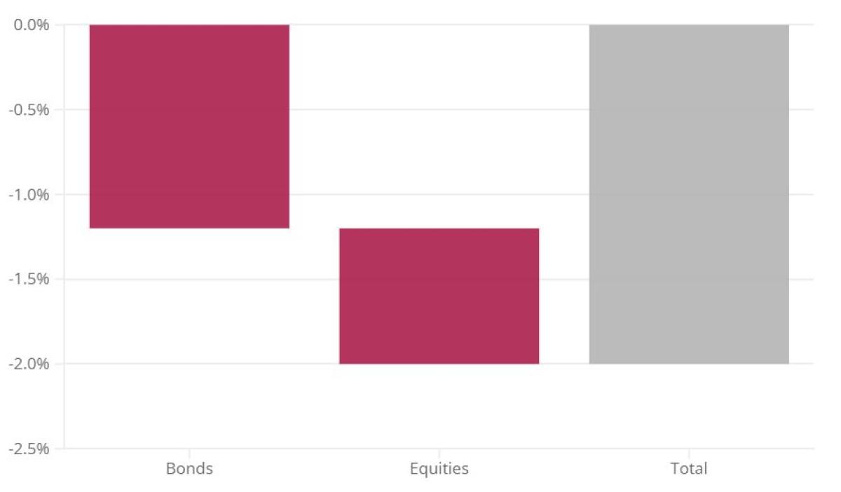
Source: Man AHL. For illustrative purposes only. Please see the important information linked at the end of this document for additional information on hypothetical results.
Monte Carlo Versus Historical Simulations
As mentioned above, the first step in calculating the tail beta is to simulate factor and portfolio returns. There are two ways in which this can be done: Monte Carlo simulation or historical.
Monte Carlo simulations will consider a forward-looking estimate of volatilities and correlations, which is typically calibrated based on recently observed volatilities and correlations. It is common to place more weight on recent observations than older observations since realized volatility and correlation tend to be ‘sticky’, i.e., if they are elevated now, they are likely to remain elevated for the next period, and vice versa.
Historical simulation, by contrast, often places equal weight on all historical days where we have returns data. Furthermore, looking in the tail of historical simulations reveals the worst outcomes in the past. These are often worse than the tail outcomes from a Monte Carlo simulation, unless the Monte Carlo simulation includes market data from a recent, particularly stressed, market environment. The historical simulation also has the advantage of being simpler and requiring fewer modelling assumptions.
Case Study
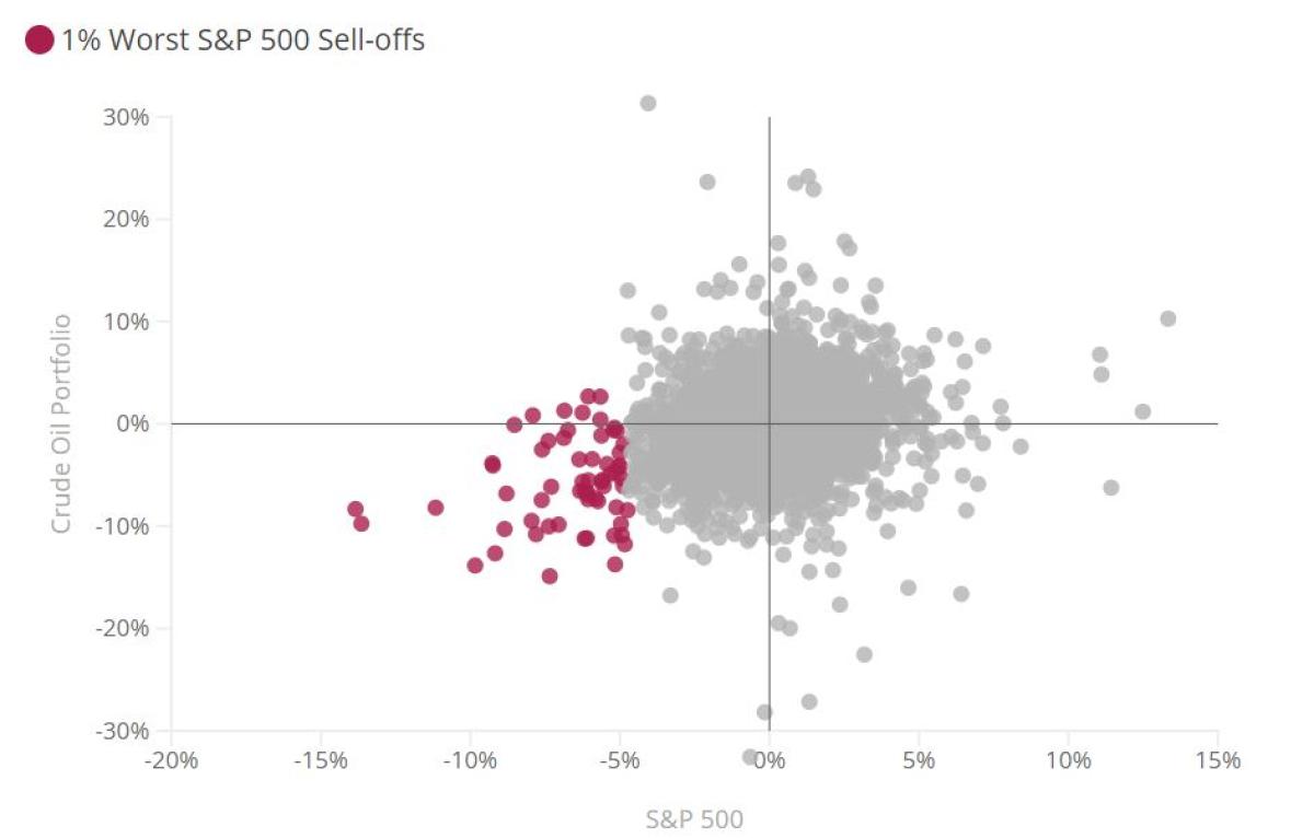
Assume a portfolio with a 100% long exposure to crude oil. A historical simulation of the portfolio’s return versus that of the S&P 500 illustrates a weak positive correlation, i.e., when the S&P 500 increased, so did the price of crude oil, resulting in a positive portfolio P&L; and vice versa (Figure 5). Indeed, on 55% of the days where the S&P 500 declined, the portfolio lost money.
However, if we look only at the 1% largest negative S&P returns, the numbers change drastically: more than 90% of the days with these large S&P 500 selloffs would have resulted in a loss for our portfolio (Figure 5, right, with worst 1% selloffs in red).
Figure 5. Correlation of Portfolio With Long Crude Oil Positions Versus S&P 500 Index
Source: Man AHL. For illustrative purposes only. Please see the important information linked at the end of this document for additional information on hypothetical results.
So, how does the ‘standard’ beta compare with the ‘tail’ beta?
Well, the portfolio beta to a 1-SD decrease (i.e., a fall of 1.7%) in the S&P 500 is -0.4%. In other words, if the S&P 500 fell a ‘typical’ 1.7%, the portfolio would lose 0.4%. In comparison, the tail beta to a 1% tail selloff (i.e., a fall of 6.6%) in the S&P 500 is -6.9% (Figure 6). The impact of moving into the tail is that the relationship between our portfolio P&L and the S&P becomes much stronger than the average relationship, because in large risk-off moves crude oil behaves more like a risk asset.
Figure 6. Impact of Portfolio P&L – Usual Beta Versus Tail Beta
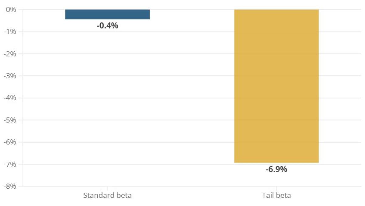
Source: Man AHL. For illustrative purposes only. Please see the important information linked at the end of this document for additional information on hypothetical results.
The Impact of Tail Betas on ‘Complicated’ Portfolios
Tail betas are a much more powerful tool when looking at ‘complicated’ portfolios, such as multi-strategy portfolios, as the correlation structure between many instruments in a long-short portfolio can break down in dramatic fashion in the tail.
This is best illustrated with an example. We’ll start with a hypothetical portfolio on a particular date that held many positions across credit, currencies, stock indices, cash equities, commodities, interest rate and volatility instruments. The reason for looking at such a complex portfolio is to examine the effect of tail dependencies across many asset classes at once.
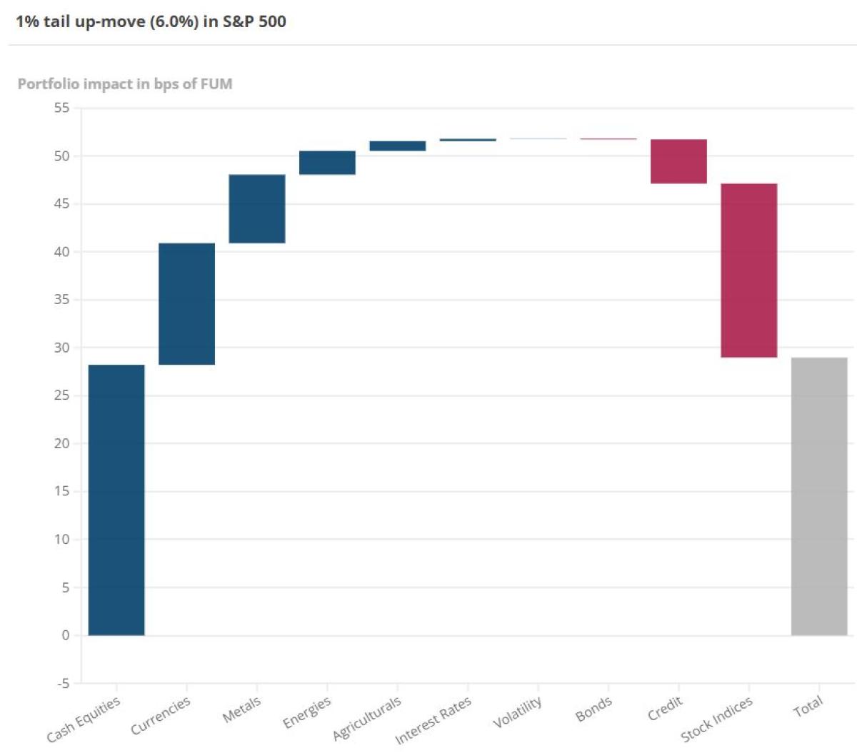
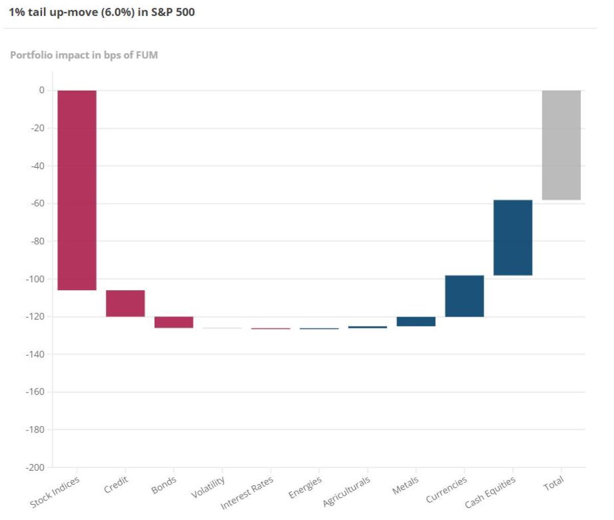
Figure 7 compares the tail betas (upper and middle charts) to the standard beta (bottom chart) for historical S&P 500 moves.
Figure 7. Tail Betas Versus Standard Betas for a Multi-Strategy Portfolio – Historical Simulation
Source: Man AHL. For illustrative purposes only. Please see the important information linked at the end of this document for additional information on hypothetical results
For the standard beta, the portfolio overall is almost completely beta neutral: if the S&P 500 rises a typical amount, the multi-strategy portfolio profits from its cash equities and bond positions, offset by losses from its commodity, credit and stock indices positioning. Overall, a ‘typical’ move in the S&P 500 has almost no expected impact on the portfolio.
The story is quite different for the tail betas to the S&P 500, especially in a down move. During the best 1% historical up-moves in the S&P 500, the portfolio returns 0.3%. During the worst 1% historical selloffs in the S&P 500, the portfolio declines 2.2%, suffering losses across every asset class except for credit. Instead of the beta-neutral portfolio we thought we had, we suffer losses on almost every single front; such is the sting in the tail.
Is There No Escape From Option Risk?
What about portfolios that feature options?
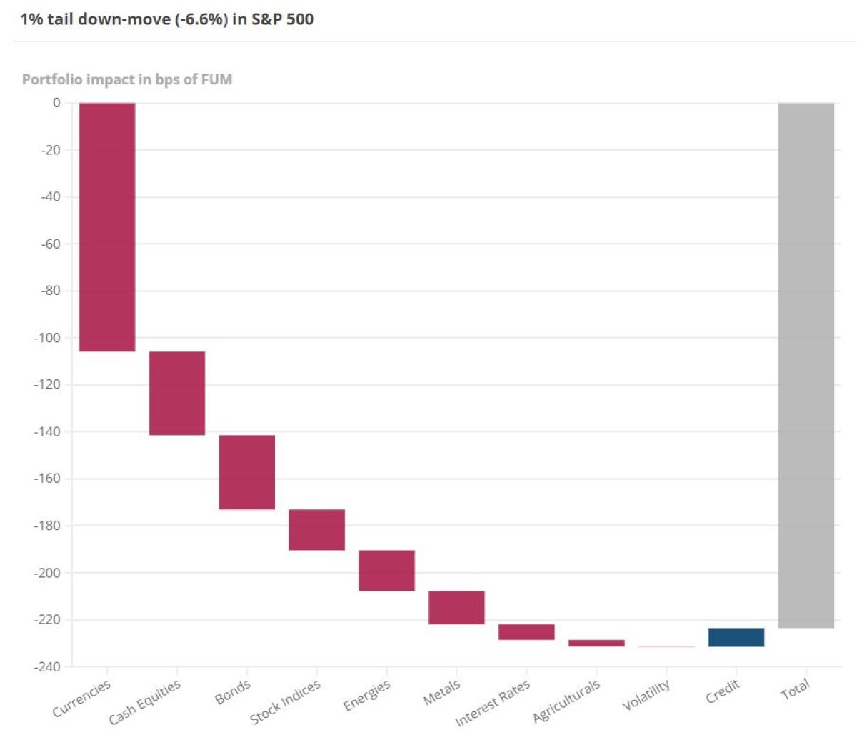
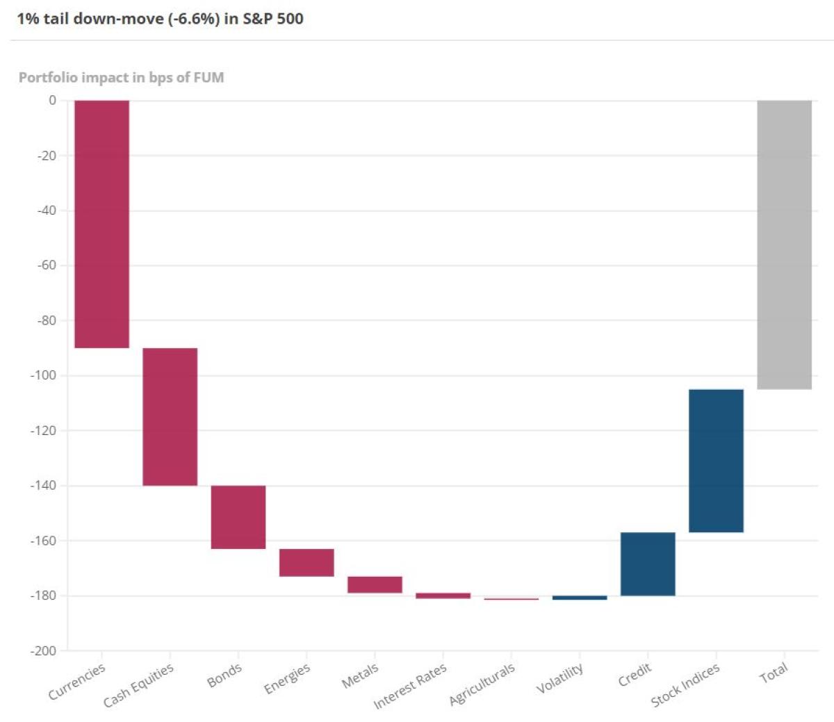
Figure 8 compares the tail betas (upper and middle charts) to the standard beta (bottom chart) for historical S&P 500 moves for a hypothetical portfolio that has options. In this example, the portfolio is mostly short gamma, which exposes the portfolio to large moves in the underlying assets, regardless of the direction of the moves.
Figure 8. Tail Betas Versus Standard Betas for a Portfolio With Options – Historical Simulation
Source: Man AHL. For illustrative purposes only. Please see the important information linked at the end of this document for additional information on hypothetical results.
For the standard beta, the portfolio returns 1.5 bps. However, similar to the multi-strategy portfolio above, the results are completely different for tail moves. Indeed, it’s bad news for the portfolio if the S&P 500 rallies (the portfolio declined by 0.6%), but it’s much worse news if the S&P 500 sells off (when the portfolio drops by 1.05%).
Figure 9 – a scatter plot of simulations used to calculate the tail betas – shows the reason why: the y-axis illustrates the P&L for the equity options in the portfolio against various-sized S&P 500 moves on the x-axis. Our overall short-gamma position results in a concave P&L: i.e., we make money with small moves in the S&P 500 but lose money in big moves.
Figure 9. P&L for Equity Options in a Portfolio Versus S&P 500 Moves
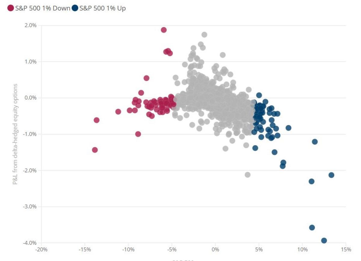
Source: Man AHL. For illustrative purposes only. Please see the important information linked at the end of this document for additional information on hypothetical results.
Another point to note here is the difference in magnitude: an average tail move in the S&P 500 is 6.6%. This is 7x as large as a typical 0.95% 1 SD move. However, because of the tail dependencies between assets and the non-linear option risk, the P&L impact on our portfolio in a tail move is about 100x the size of the P&L impact in a typical move in the S&P 500.
Conclusion
Tail betas enable investors to understand the hidden risks within their portfolios, especially during extreme moves in financial markets. Indeed, tail betas shine a light on breakdowns in correlation structure, skewness and asymmetry of returns, and heavy-tailed returns, none of which are considered by standard betas calculated using linear regression or a covariance matrix.
While tail betas aren’t a panacea, as they still assume all possible moves are captured in the historical data or Monte Carlo models used, they are nonetheless a powerful tool for risk management of portfolios and can help investors potentially avoid the sting of the tail.
Footnotes:
1. www.cnbc.com/2021/12/05/market-history-says-omicron-volatility-isnt-a-reason-to-sell.html
2. Source: Bloomberg.
3. Our definition of factor is generalizable to any timeseries data – it could be an index, an asset, or an economic factor such as the GDP of a country. See our previous explanation of betas here: How to Calculate the Beta of a Portfolio to a Factor
About the Authors:
Oliver Whitehead is Head of Investment Risk at Man AHL.

Prior to joining Man AHL in 2018, Oliver worked for Bank of America Merrill Lynch, where he was most recently a risk manager, responsible for a number of fixed-income trading desks. Before that, he worked as a quantitative analyst developing new risk and pricing models. Oliver holds an integrated Master’s degree in Mathematics from the University of Warwick.
John Townhill is a quant on the Investment Risk team at Man AHL, responsible for monitoring and managing risk across Man AHL portfolios.

Prior to joining Man AHL in 2021, John worked for an actuarial consultancy. John holds an integrated master’s degree in Mathematics from the University of Oxford and is a Fellow of the Institute of Actuaries.