


By Dan diBartolomeo, President and founder of Northfield Information Services, Inc. Based in Boston since 1986, Northfield develops quantitative models of financial markets.
In recent years, global equity markets have experienced episodes of extreme volatility over short periods. When this happens, our “near horizon” models can begin predicting risk values higher than our “long horizon” models.
The traditional formulation of Modern Portfolio Theory is a single period model where our beliefs about the distributions and correlations of asset returns are fixed. Essentially, there are only two concepts of time, now and the end of time. In the real-world market conditions change from day to day and year to year. These changes are often of great magnitude. Our first challenge will be deal with the changing levels of risk over time.
MPT also assumes that all assets are completely liquid, so transaction costs are zero. Again, in the real-world transaction costs are not zero and in crisis conditions are often extremely large. Our second challenge will be to form a more realistic framework for this issue.
Time Horizon and Risk Assessment
It is the common practice of the investment industry to discuss portfolio return volatility in annual time units. We say “the implied volatility of a stock option is 30 percent per year,” or “the tracking error of a portfolio is 3 percent per year.” But it is unclear whether we really are assessing the expectation of volatility between today and one year from today or if we are describing the annualized value of volatility over some shorter (or longer) period such as the next week or month. Much of the variation in risk assessment provided by various widely used risk systems arises from this ambiguity.
We must address two more issues when we consider time horizons. The first is that the statistical measures that use portfolio volatility can be translated into probabilities of gain or loss in two different ways. The usual approach is to consider the distribution of portfolio values at the end of the horizon period. Let’s assume we have a portfolio worth $1 million with an expected return of zero and a volatility of 10 percent per annum.
We will further assume that the returns are normal and are independently and identically distributed (no serial correlation and constant volatility). In such a case, a three-standard-deviation event downward would equate to a 30-percent loss reducing the portfolio value to $700,000 at the end of the one-year period. The likelihood of such an occurrence is about one in 1,000. Investors often confuse this with the probability that the value of the portfolio will never go below $700,000 at any point during the year. We call this risk the “first passage” potential for loss compared to the “end of horizon” potential for loss. Because there is always some chance that the portfolio could fall below the floor of $700,000 at some point during the year yet still end the year at about $700,000, the first-passage probability of given loss is greater than the probability of the comparable end-of-horizon loss.
As described in Kritzman and Rich (2002), under the most typical assumptions one can express the intra-horizon probability of hitting the boundary value as:
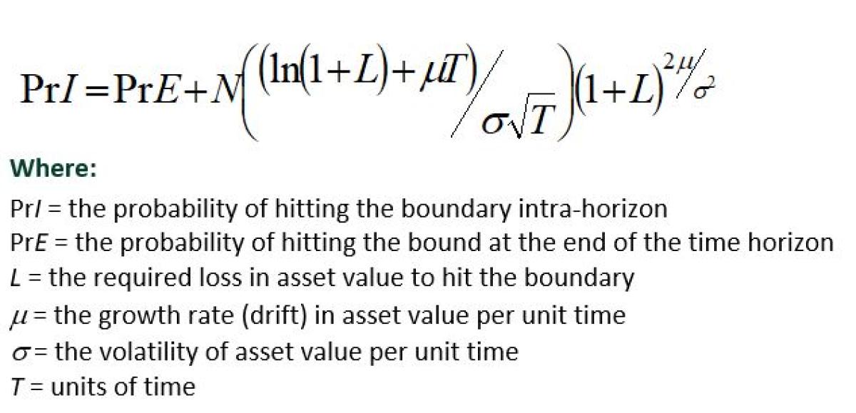
Another way of thinking of this problem is to ask how much we would have to reduce the volatility of the portfolio so that the probability of a first-passage loss at the floor would equal the end-of-horizon probability of the same loss, given the original portfolio volatility. In the case of our simple example portfolio above with volatility 10 percent, we would have to reduce the portfolio volatility to 9 percent (i.e., 10/1.11) to get the same roughly one in 1,000 chance of having the portfolio value go below $700,000 at any time during the year. Numerous papers such as Feller (1971) and Bakshi and Panayatov (2010) suggest scaling divisors ranging from roughly 1.11 to 2.64 depending on the type of assumed return process (normal, independent and identically distributed, jumps, stochastic volatility, etc.).
The other issue we must deal with when considering first-passage risk is that the shape of the return distribution may be different depending on whether we are measuring returns on a daily (or intraday) basis or on a monthly or annual basis. In general, the shorter the observation interval (i.e., the higher the observation frequency), the greater the tendency of the observed return distribution to have “fat tails,” meaning that extreme moves up or down are much more frequent than predicted in a normal distribution. An extensive review of this issue is provided by diBartolomeo (2007). To the extent we believe that the returns for our portfolio will be fat-tailed we can choose higher values of the scaling divisors described above to compensate. The usual approach for determining the magnitude of the adjustment is the Cornish-Fisher (1937) expansion method.
Conditional Risk Models
Our second weapon to address the time-varying nature of risk is to build risk models that adapt more rapidly to changes in market conditions. The traditional approach to this process is to build the risk model with data observed over a shorter window of history but with a higher frequency of observations. As described in diBartolomeo (2007), high-frequency data often has undesirable statistical properties that make estimating such models reliably almost impossible.
A different approach is embodied in the concept of conditional models that are based on a vector of state variables. Rather than simply build our model based on our observations of the past, we can also include information that is observable right now. Northfield has used the conditional model concept in our US Short-Term model since 1999, and “near horizon” versions of all of our risk models have been available since April of 2009.
This approach allows any chosen model to adapt rapidly to changes in market conditions, but to retain the existing factor definitions and factor exposures. In effect, we ask ourselves how market conditions today are different than they were on average during the period of history used to estimate the usual model. To judge the degree of difference, an information set of state variables are defined that describe contemporaneous aspects of the financial conditions but that are not normally used in the risk model. Such variables might include the implied volatility of options on stock indexes (e.g., VIX) and bond futures, yield spreads between different credit qualities of bonds, and the cross-sectional dispersion of stock returns among different sectors and countries.
In mathematical terms, we can think of this process as built around a vector we’ll call theta. For each important element of the risk model (e.g., the volatility of a factor), there will be a corresponding element in the vector theta. Each element of the vector has a default value of one. We multiply each element of the model by its corresponding element in theta in order to reflect changes in state variables. For example, if a firm’s manufacturing plant were to be destroyed in a flood, it would take many observations of returns to make a new estimate of how the covariance of this firm with returns of other firms had changed due to the changed circumstances.
However, if the firm in question had traded options, we might immediately observe a change in the stock volatility implied by the prices of the traded options. The relative change in the implied volatility as compared to past values of implied volatility would be reflected in the theta vector and could help to immediately adjust our risk expectations for this firm, as described in diBartolomeo and Warrick (2005), and refined in Shah (2008).
Using news itself to condition factor risk estimates has also been explored recently. In diBartolomeo, Mitra and Mitra (2009), the content of textual news flows through a news service (e.g. Dow Jones, Bloomberg, Reuters) is analyzed for length, frequency and sentiment. They conclude that conditioning on news content add meaningfully to the responsiveness of risk estimates, even beyond the use of implied volatility for securities with liquidly traded options.
To illustrate how the conditional risk model concept works, we took an example portfolio of 50 stocks drawn at random from the S&P 500 at August 31, 2011. All stocks were equally weighted. We then use our “regular” and “near horizon” US Fundamental Model to make tracking error (against the S&P 500 as benchmark) and absolute risk assessments. During the period from March 31st, 2011 to September 15th, 2011 the tracking error estimates using our usual one-year time horizon ranged from a low of 5.07% to a high of 5.89%. Over the same span, the value of forecast absolute portfolio volatility ranged from a low of 24.34% to a high of 25.52%. It should be noted that the high and low values for tracking and error and absolute volatility are not necessarily coincident in time.
The “near horizon” version of the US Fundamental Model has a forecast time horizon of ten trading days. When we evaluated the same portfolio using the near horizon version, we get a very different picture. For example, at April 15th, 2011, before most of the volatility inducing events had occurred the near horizon “annualized” tracking error estimate was 3.79% and the absolute volatility value was 14.80%. The lower values show that the near horizon model was paying more attention to the relatively benign post crisis conditions than the longer-term model up to April 15th. By the 13th of September, the tracking error estimate had risen to 5.52% but the absolute risk estimate was 30.45%.
Liquidity Risk
As most institutional investors are exempt from taxes, it is customary to think of investment portfolios in terms of total return. The distinctions between income and capital growth and between the market value of a portfolio and actual spendable cash are forgotten. For our purposes, let us consider liquidity risks as being those related to the potential to have to bear excessive costs to convert an investment asset into cash available for consumption spending.
The first aspects of liquidity risk to consider are structural impediments. For example, many charitable foundations are legally limited to spending only the income (interest and dividends) derived from their investment portfolio but are not permitted to liquidate portfolio assets into cash for consumption. A less restrictive form of this constraint would be the situation where an endowment can spend income for consumption and also liquidate appreciated assets as long as the market value of the portfolio never declines below the original value of the capital contributed.
Regulators of financial services firms often impose liquidity requirements. For example, the insurance regulators in some European countries require that insurance portfolios contain an amount of very liquid assets (cash and government bonds) to cover the expected claims for the next three years. The assumption here is that over a three-year span even illiquid investments such as exotic fixed income securities, real estate and private equity partnerships can be converted to cash without resorting to drastic “fire sale” discounts as were seen in mortgage derivative securities during the recent global financial crisis.
There is a very tractable way to adjust traditional portfolio risk metrics (volatility, tracking error, VaR) to reflect liquidity concerns. We begin by getting the investor to state a liquidity policy as described in Acerbi and Scandolo (2008). Once our policy is stated we can calculate the cost of a hypothetical liquidation and then build the associated transaction costs into the portfolio risk estimates.
To do this we convert our portfolio volatility estimate to parametric Value-at-Risk for the length of time specified in our liquidity policy. We can then add the expected cost of a potential liquidation to the VaR value, and convert the VaR value back to the equivalent volatility. For example, let us assume that we must be able to liquidate 30% of the portfolio in 10 trading days that our estimated portfolio volatility is 25% per year, and that the expected cost of carrying out the liquidation would be 4% of the portfolio value (12% of the 30% to be converted to cash). A profound result of this kind of analysis is that portfolio risk is a function, not only of portfolio weights but also of the dollar value of the portfolio, as the larger the positions are the greater the expected costs of liquidation will be. This means that a $1 Billion portfolio is riskier than a $1 Million portfolio even if the security composition and weights are identical.
Under the common parametric assumptions, we can estimate the portfolio volatility measure (probably using a factor model) and then algebraically convert the volatility value to the VaR or CVaR. Given that solvency-based risk management is a day-to-day affair, we must be aware of the “fat tail” issues previously mentioned. To adjust the normal distribution assumption for “fat tails” we can use the Cornish Fisher expansion method (1937) to rescale the volatility value. Alternatively, we could assume that the distribution of asset returns has a fat tailed distribution (e.g., Gamma, Weibull). For the common case of the normal distribution assumption, the transform is:
VaR$(p,t) = V * sf * (t/250).5 * Z(p)
Where:
V = the dollar value of the portfolio
sf = annualized volatility of the portfolio adjusted for fat tails
t = the number of days to the forecast horizon
Z(p) = number of standard deviations below the mean for the cumulative density of P%
For sake of simplicity, we will use a 3-standard deviation VaR which covers 99.8% of the density of a normal distribution. In such a case our % parametric VaR would be 14.94% [25 * 3 * (10/252).5]. If we now add our forecast liquidation cost of 4%, we get a revised % parametric VaR of 18.94% [14.94 + 4]. By reversing our arithmetic, we can convert back to the equivalent value of volatility, 31.70 [18.94 / 3 * (252/10).5]. In our example, the portfolio volatility estimate increased from 25% annually to 31.7%. The increase in variance is from 625%2 to 1005%2.The 380 unit increase in variance is apt to reduce the geometric mean return by 1.9% relative to the arithmetic mean.
In some sense, a “growth optimal” investor is apt to be more satisfied with this somewhat illiquid portfolio if and only the expected return is at least 1.9% per annum more than a completely liquid portfolio of comparable market risk. Investors who are more conservative than growth optimal, even larger return premiums would be needed to compensate for the liquidity risk. Conversely, in estimating an economically appropriate return premium for liquidity, we must also keep in mind that the probability of having to actually carry out a liquidation process is apt to be substantially less than one.
The Northfield/CQF Video Course on Investment Risk is Now Available. This is a ten-episode educational video series produced by Northfield and the CQF Institute. Hosted by Dan diBartolomeo.
References
Bakshi, G., and G. Panayatov. 2010. “First-Passage Probability, Jump Models, and Intra-Horizon Risk”, Journal of Financial Engineering 95, no. 1 (January): 20–40.
Cornish, E., and R. Fisher. 1937. “Moments and Cumulants in the Specification of Distributions.”, Extrait de la Revue de l’Institute International de Statistique : 1–14.
diBartolomeo, Dan. 2007. “Fat Tails, Tall Tales, Puppy Dog Tails.” Professional Investor, Autumn.
Feller, W. 1971. An Introduction to Probability Theory and Its Applications, Vol. II. (New York: John Wiley & Sons, Inc.)
Kritzman, Mark and Don Rich, 2002. The Mismeasurement of risk. Financial Analysts Journal 58, 91-99.
Acerbi, Carlo and Giacomo Scancolo. 2008. “Liquidity Risk Theory and Coherent Measures of Risk”, Quantitative Finance.
All posts are the opinion of the contributing author. As such, they should not be construed as investment advice, nor do the opinions expressed necessarily reflect the views of CAIA Association or the author’s employer.
About the Author:
Mr. diBartolomeo is President and founder of Northfield Information Services, Inc. Based in Boston since 1986, Northfield develops quantitative models of financial markets. The firm’s clients include more than one hundred financial institutions in a dozen countries.

Dan serves on the Board of Directors of the Chicago Quantitative Alliance and is an active member of the Financial Management Association, (“QWAFAFEW”), the Society of Quantitative Analysts. Mr. diBartolomeo is a Director of the American Computer Foundation, a former member of the Board of Directors of The Boston Computer Society, and formerly served on the industry liaison committee of the Department of Statistics and Actuarial Sciences at New Jersey Institute of Technology.
Dan is a Trustee of Woodbury College, Montpelier, VT and continues his several years of service as a judge in the Moscowitz Prize competition, given for excellence in academic research on socially responsible investing. He has published extensively on SRI, including a forthcoming book (with Jarrod Wilcox and Jeffrey Horvitz) on portfolio management for high net-worth individuals.