Hedge Fund Due Diligence With Factor Model Monte Carlo

By Aric Light, Relationship Manager at Merrill Lynch where he advises high net-worth families and institutions.

1. Introduction

Due diligence for hedge funds presents a unique set of challenges for analysts and asset allocators. Funds often have significant discretion to invest across multiple asset classes and instruments and deploy strategies of varying complexity ranging from well-known approaches such as equity long-short to more exotic schemes like capital-structure arbitrage. Funds may also deal in highly illiquid markets with holdings that are either marked to market infrequently or marked to models that are generally not made available for inspection.  Indeed, Hedge Fund Research tracks indices for at least 70 unique hedge fund strategies. The breadth of strategies available requires plan sponsors to carefully select which assets they want exposure to without inadvertently concentrating in any one source of risk.

Such dynamics introduce opacity into an already challenging process. As such, it is crucial for allocators to have a rigorous, quantitative framework for benchmarking performance and measuring risk. In this post, I’ll review the use of Factor Model Monte Carlo (FMMC) simulation as a general and robust framework for assessing the risk-return drivers of hedge fund strategies. We’ll find that FMMC has many attractive qualities in terms of implementation and offers highly accurate estimates of several commonly used risk and performance metrics. The hope is that this post provides plan consultants, boards and trustees with a useful and intuitive tool to complement their due diligence process for hedge funds.

2. Task and Setup

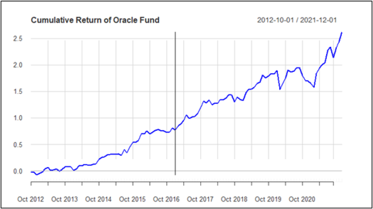
To demonstrate the efficacy of the Factor Model Monte Carlo approach we will be applying the methodology to the real-world example of Oracle Fund. The name Oracle Fund is fictious, but the returns are very real. Oracle is an active, investable fund made available only to Qualified Purchasers (i.e., investors with a net-worth in excess of $5MM) hence the anonymized name.

By way of background, Oracle is managed by a very well-known investment advisor with ~$140B in AUM. Oracle is described a long-short equity fund with the stated investment objective of providing “equity-like” returns with lower volatility by systematically investing in stocks that are:

• Defensive: low market beta
• High Quality: strong balance sheets and consistent cash flow generation
• Cheap: relatively lower multiples

The strategy invests in developed market public equities with an investable universe containing ~2,300 large cap and ~2,700 small cap stocks.

For this case study we have access to monthly return data for Oracle from October 2012 through December 2021. However, for the purpose of this post and evaluating the accuracy of the model we will pretend as though we only have data from January 2017 through December 2021. The purpose of using the “truncated” time series is threefold. First, by estimating our model using only half the available data we can perform “walk forward” (walk-backward?) analysis to evaluate how well our estimates match those from the out of sample period. Second, measuring risk-return over a single market cycle may lead us to bias conclusions. By breaking up the sample period we can see how well our results translate to other market environments. Third, in the case of evaluating a new or emerging manager only a short history of returns may be available for analysis. In such a case, it is essential to have a reliable tool to project how that manager may have performed under different circumstances.

The below graph shows the cumulative return of Oracle since October 2012. The data to the right of the red line represents the “sample period”.

1. Model Specification and Estimation

A common technique in empirical finance is to explain changes in asset prices based on a set of common risk factors. The simplest and most well-known factor model is the Capital Asset Pricing Model (CAPM) of William Sharpe. The CAPM is specified as follows:

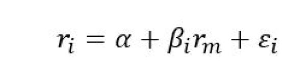
Market risk, or “systematic” risk, serves as a kind of summary measure for all of the risks to which financial assets are exposed. This may include recessions, inflation, changes in interest rates, political turmoil, natural disasters, etc. Market risk is usually proxied by the returns on a large index like the S&P 500 and cannot be reduced through diversification. (i.e. Beta) represents an asset’s exposure to market risk. A Beta = 1 would imply that the asset is as risky as the market, Beta >1 would imply more risk than the market, while a Beta < 1 would imply less risk. is idiosyncratic risk and represents the portion of the return that cannot be explained by the Market Risk factor.

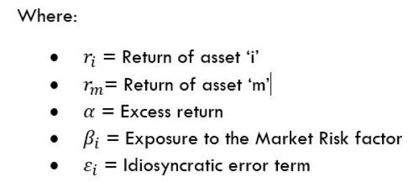
As a long-short hedge fund, part of Oracle’s value proposition is to eliminate some (or most) of the exposure to pure market Beta (otherwise, why invest in a hedge fund?). Thus, we will extend CAPM to include additional risk factors which the literature has shown to be important for explaining asset returns.

The general form of our factor model is as follows:

All the above says is that returns (r) are explained by a set of risk factors j=1…k where rj is the return for factor ‘j’ and βj is the exposure. ε is the idiosyncratic error.

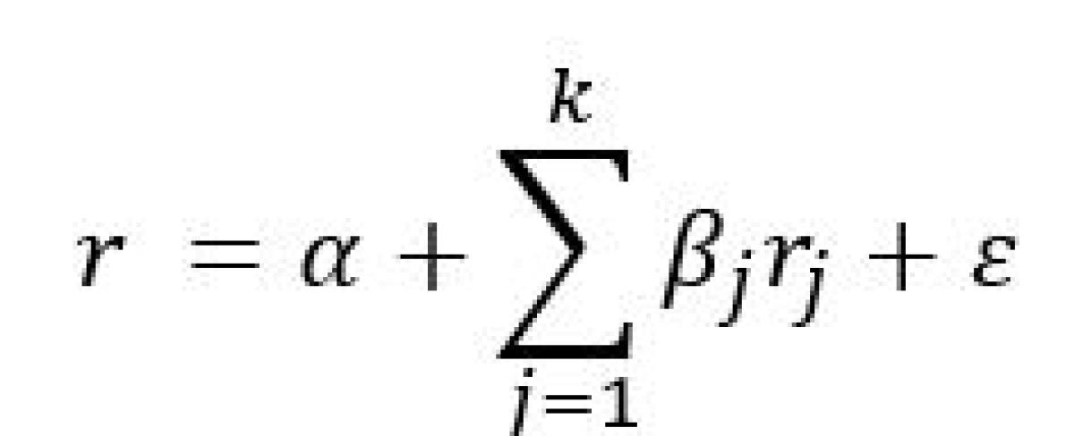
Thus, if we can estimate the βj, then we can leverage the long history of factor returns (rj) that we have and calculate conditional returns for Oracle’s. Finally, if we can reasonably estimate the distribution of ε then we can build randomness into Oracle’s return series (more on this in a bit). This enables us to fully capture the variety of returns that we could observe.

The FMMC method will take place in three parts:

• Part A: Data Acquisition, Clean Up and Processing
• Part B: Model Estimation
• Part C: Monte Carlo Simulation

Part A: Data Acquisition

Part of the art of analysis is selecting which set of variables to include in a model. For this study, I will be examining a set of financial and economic indices aimed at capturing different investment styles and sources of risk/return. Below is the list of variables. Economic time series were obtained from the FRED Database (identifier included in paratheses), financial indices were obtained from Yahoo! Finance and hedge fund index returns come courtesy of Hedge Fund Research. Somewhat surprisingly the HFR indices are freely available for download by the investing public on their website (you must register and create a login, but still…this level of detail for free is rather generous).

• Term premium: Yield spread between 3-month and 10-year Treasuries (T10Y3M)
• Credit Spread: Moody's Baa corp. bond yield minus 10-year Treasury yield (BAA10Y)
• 3-month T-Bill Rate (DGS3MO)
• TED Spread: 3-Month LIBOR Minus 3-Month Treasury Yield (TEDRATE)
• BofAML Corporate Bond Total Return Index (BAMLCC0A0CMTRIV)
• 10-Year Inflation Expectations (T10YIE)
• Russell 1000 Value
• Russell 1000 Growth
• Russell 2000
• S&P 500
• MSCI EAFE
• Barclays Aggregate Bond Index
• HFRI Equity Market Neutral
• HFRI Fundamental Growth
• HFRI Fundamental Value
• HFRI Long-Short Directional
• HFRI Quantitative Directional
• HFRI Emerging Market China
• HFRI Event Driven Directional
• HFRI Event Driven – Total
• HFRI Japan
• HFRI Global Marco – Total
• HFRI Relative Value - Total
• HFRI Pan Europe

Part B: Model Estimation

Recall that for this case study we are “pretending” as though we only have returns data for Oracle from January 2017 through December 2021 (i.e., the sample period). In reality, we have data going back to October 2012. We will use the data in the sample period to calibrate the factor model and then compare the results from the simulation to the long-run risk and performance over the full period.

Model estimation has 2-steps:

1. Estimate a Factor Model: Using the common “short” history of asset and factor returns, compute a factor model with intercept α, factor betas βj for j=1…k, and residuals ε.
2. Estimate Error Density: Use the residuals ε from the factor model to fit a suitable density function from which we can draw.

Estimation of the error density in Step 2 presents a challenge. One approach is to fit a parametric distribution to the data. This is a one-dimensional problem and, in theory, may be done reasonably well by using a fat-tailed or skewed distribution. However, such an approach has to potential to introduce error into the modeling process if the wrong distribution is chosen. Moreover, in the case of a short return history there simply may not be enough data available to fit a suitable density.

To get around the need for a parametric distribution, we will instead use the empirical or “non-parametric” estimates of the probability distribution of errors which we can easily obtain once we have estimated the calibrated model for the short “sample” period. This method enables us to reuse residuals that were actually observed, capture potential non-linearities in the data and model behavior at least fairly far out into the tails.

Having charted a path forward for dealing with the error distribution, we can now proceed to estimating the factor model. I have proposed 24 candidate variables to explain the returns of Oracle, but I don’t know which ones offer the best fit. It would be bad statistics to run a 24 variable regression and see what happens; what we want is an elegant model that uses a subset of the proposed. A typical approach to this problem is to minimize an objective function such as the Akaike Information Criterion (AIC) or Bayesian Information Criterion (BIC). In general, it is often possible to improve the fit of a model by adding parameters but doing so may result in overfitting. Both BIC and AIC attempt to resolve this problem by introducing a penalty term for the number of parameters in the model; with the BIC penalty being larger relative to AIC.

We’ll define the BIC as follows:

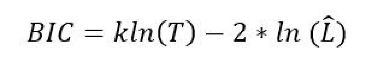
Where:

• k = # of model parameters including the intercept
• T = sample size
• L = the value of the likelihood function

To find the model that minimizes the BIC I used the regsubsets function available in the leaps package in R. regsubsets uses an exhaustive search selection algorithm to find the model which minimizes the BIC. I set the “nvmax” parameter (i.e., the maximum number of variables per model) to 15. The selection algorithm returned the following 5 factor model:

• S&P 500 (i.e., the Market Risk Factor)
• HFRI Equity Long Short Directional Index
• HFRI Japan Index
• HFRI Global Macro Index – Total
• Term Premium

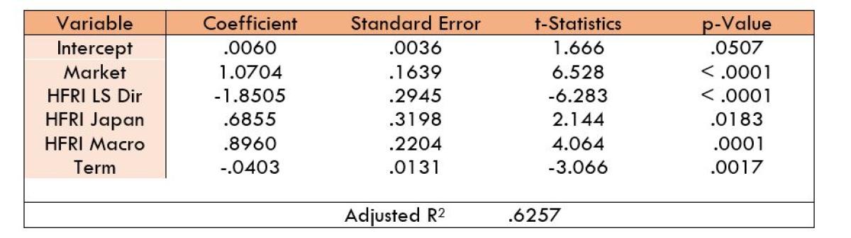
Below are the regression results. Standard errors have been adjusted for heteroscedasticity and autocorrelation.

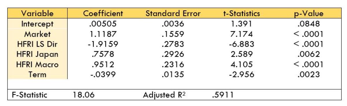
I think it is worth noting how parsimonious the model is. We have distilled the sources of macro-financial risk for Oracle down to just 5 components. As previously stated, Oracle pursues a developed markets directional equity long-short strategy so we would expect equity factors to feature prominently. Except for the Term premium all the other factors are equity based. This is good! Had the model returned significant results for the Barclays Aggregate Bond Index or Emerging Markets China then we might have cause for concern that the manager is not pursing the strategy as advertised.

The Market risk factor (as proxied by the S&P 500) is highly statistically significant and of the sign we would expect as Oracle has a long bias. HFRI Japan is also positive and significant which speaks to the strategy’s global developed markets approach. The HFRI Long-Short Directional Index is significant as we would hope for a fund that markets itself as, you know, equity long-short! However, the sign is a little hard to interpret. I had anticipated this variable to be positive. One possible explanation for the negative coefficient is that most funds which comprise the index were on the other side of the trade over the sample period. It would be appropriate to describe Oracle’s strategy as titled toward value (i.e., defensive stocks, low multiples, low beta). Over the last decade a popular hedge fund strategy has been long growth and short value, which was quite lucrative for some time, but in 2022 has turned disastrous. If this is the case, then it makes sense for Oracle to have significant, but negative exposure to this risk factor.

The adjusted-R² of .5911 suggests that ~60% of the variability in Oracle’s return is explained by the model risk factors. The below plot illustrates the realized returns of Oracle and the fitted values from the calibration period January 2017 – December 2021:

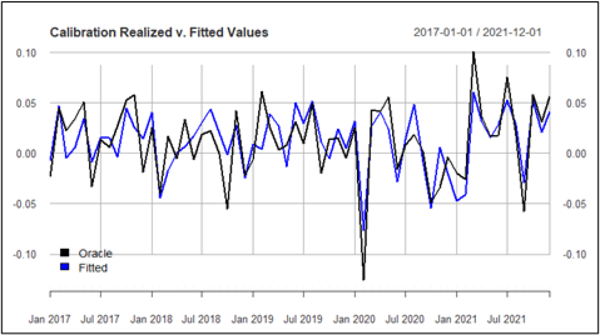
Maximizing R² is typically not a recommended practice which is why we used the BIC as our selection criterion. On balance, an R² of ~.60 suggests a reasonable degree of explanatory power, but tighter would be better. This moderate fit could be because we have neglected to include important variables in our modeling process or Oracle has some “secret sauce” which is not captured by the variables. The other explanation is the potentially troublesome presence of outliers.

Influential Points and Outlier Detection

To identify outliers, we can use a combination of visual and statistical diagnostics. These methods include Cook’s Distance (Cook’s D), leverage plots, differential betas (DFBETAS), differential fits (DFFITS), and the COVRATIO (pronounced “cove” ratio). For conciseness (and because this isn’t a post about outlier detection) we’ll focus on just two measures: DFFITS and COVRATIO. 

DFFITS is defined as the difference between the predicted value for a point when that point is left in during the regression estimation v. when that point is removed. DFFITS is usually presented as a studentized measure. I think the formula makes this definition more digestible:

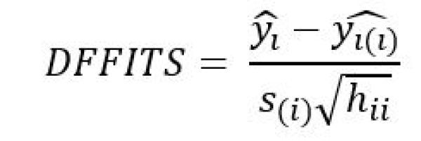
Where:

• y_i = prediction for point ‘i’ with point ‘i’ left in the regression
• y_i(i) = prediction for point ‘i’ with point ‘i’ removed from the regression
• s_(i) = standard error for the regression with point ‘i’ removed from the regression
• h_ii = is the leverage for point ‘i’ taken from the “hat” matrix 

The developers of DFFITS have suggested using a critical value of 2pn to identify influential observations; where ‘p’ is the number of parameters and ‘n’ is the number of points. The calibrated model has 6 parameters (5 variables plus the intercept) and 60 points which gives us a critical value of .63.

We can plot the results of DFFITS to help visually identify influential data as seen in the below chart.

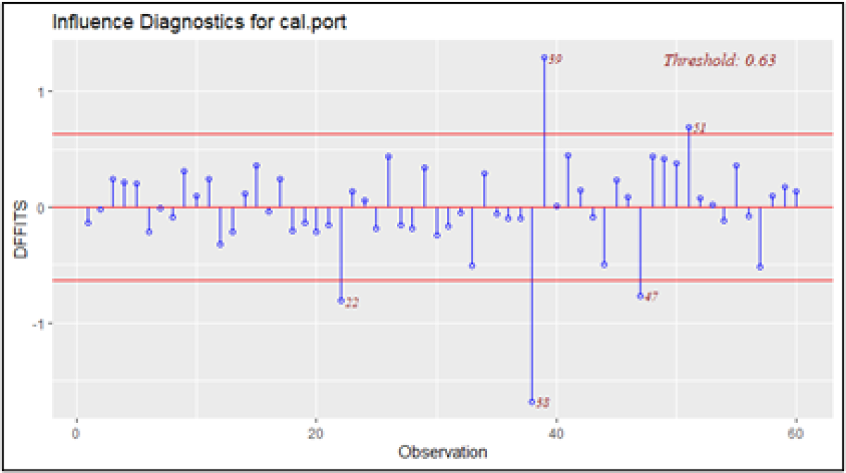
The plot shows that 5 points exceed the critical threshold of .63 with observations 38 and 39 standing out in particular. As you might have guessed, these two points correspond to February and March 2020, respectively.

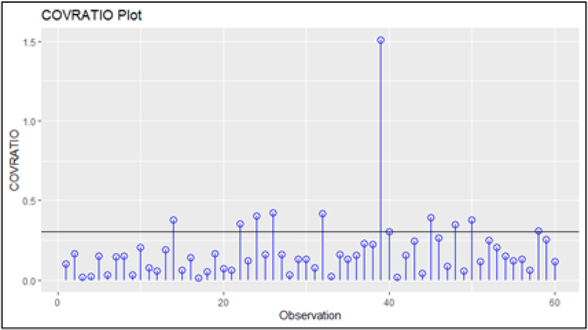
We can use the COVRATIO to corroborate the results from DFFITS. The COVRATIO measures the ratio of the determinant of covariance matrix with the i^th observation deleted and the determinant of the covariance matrix with all observations.

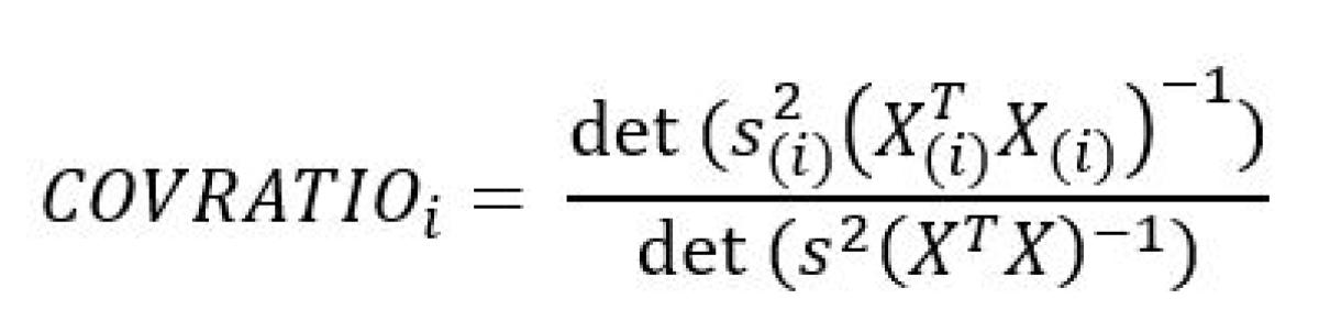
Values for the COVRATIO near 1 indicate that the observation has little impact on the parameters estimates. An observation where COVRATIO-1> 3pn is indicative of an influential datapoint.

The results from the COVRATIO returned 10 potentially influential points; see plot. Taken together with results from DFFITS we can comfortably conclude that our model is subject to the effects of outliers. If we are to build a model that will perform well out of sample, then it is critical to have robust parameter estimates that we are confident capture the return process of Oracle across different time periods. Enter robust regression.

Refining our Factor Model with Robust Regression

Having identified the outliers in our dataset, we can attempt to mitigate the impact these observations have on our parameter estimates by rerunning the factor model regression on reweighted data in a process referred to as robust regression.

Several weighted schemes have been proposed for dealing with influential data, but the two most popular are the Tukey Biweight and Huber M estimators. Huber’s M estimator reweights the data based on the following calculation:

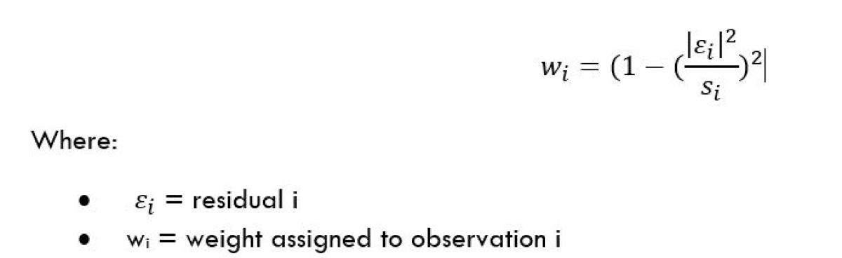
The basic intuition is that the larger the estimated residual, the smaller the weight assigned to that observation. This should consequently reduce the impact of outliers on the regression coefficients and (hopefully) stabilize the estimates such that we can apply them out of sample.

The below table gives the factor model using Huber estimation:

The results from the reestimated model are broadly similar to the initial OLS estimates with the coefficients of HFRI Japan and HFRI Macro exhibiting the most notable change. The R-squared has marginally improved from ~.59 to ~.62, but practically speaking this is the same degree of fit. Overall, OLS and Huber are communicating the same basic results.

As we press forward to the simulation results in the next section (finally!) we’ll adopt the Huber model as the factor model which we will use to forecast risk and return estimates for Oracle.

Part C: Simulation

The goal of this study is to accurately estimate the risk and performance profile of Oracle Fund using Monte Carlo simulation; all the better if we can do it efficiently. As noted in Part B, when it comes to Monte Carlo simulation there are two standard approaches: parametric and non-parametric. Parametric estimation requires that we fit a joint probability distribution to the history of factor returns from which to draw observations. This is a challenging problem as it requires us to estimate many (and quite likely, different) fat-tailed distributions and a suitable correlation structure. While this is theoretically achievable, it is best avoided in our case.

Instead, we can use the discrete empirical distributions from the common history of factor returns as a proxy for the true densities. We can then conduct bootstrap resampling on the factor densities where a probability of 1/T is assigned to each of the observed factor returns for t=1…T. Similarly, we can bootstrap the empirical error distribution from the residuals we obtained from the estimated factor model in Part B. In this way we can reconstruct may alternative histories of factor returns and errors. Proceeding in the way should enable us to gaze relatively far into the tails of risk/return profile for Oracle and better understand the overall exposure to sources of systematic and idiosyncratic risk.

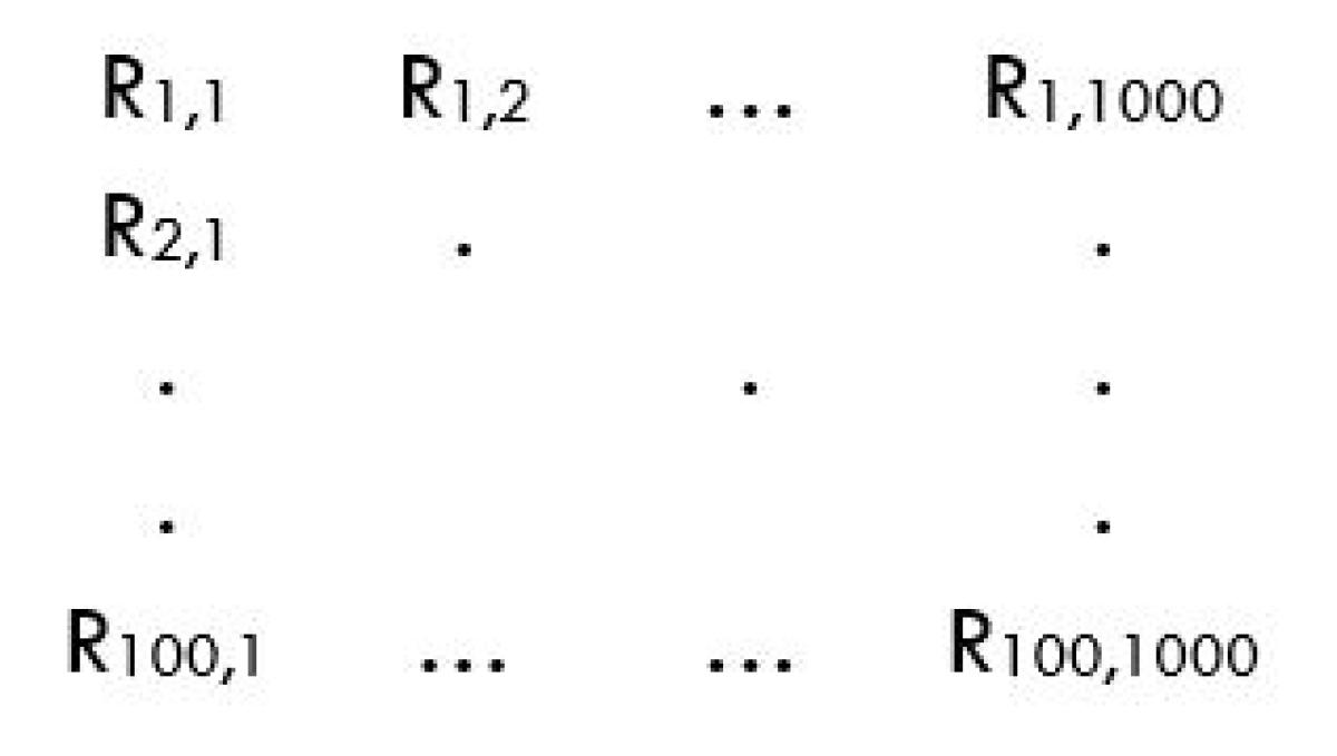
For this simulation I conducted 1000 bootstrap resamples each of size 100. The steps were as follows:

• For iteration i…1000 (i.e., column i), observation j…100 (i.e., row j) randomly sample a row of factor returns from the factor return matrix and error estimate from the empirical error distribution.
• Plug these values into the factor model from Part B to form an estimate for Oracle’s return for the i^th, j^th period.

The resultant matrix of estimated returns for Oracle should appear as follows:

Performance Analysis

Alright…after all of that hard work we have finally come to the fun part: performance! To recap our setting, recall that the full performance history for Oracle spans October 2012-December 2021. Thus far we have pretended as though we only have returns for January 2017-December 2021 (i.e., the sample period). We have used the common short history of factor returns to estimate a factor model to describe Oracle’s return process and obtained the residuals. We conducted bootstrap resampling of the short history (i.e., January 2017-December 2021) of factor returns and residuals to estimate 1000 different return paths each of size 100.

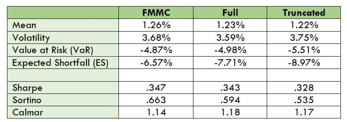
We can now use these 1000 return paths to estimate risk and performance metrics and compare the results across 2 different time scales:

• Full period: October 2012-December 2021
• Truncated period: October 2012-December 2016

This should provide us with a fairly comprehensive basis for which to evaluate the factor model Monte Carlo (FMMC) methodology.

The below table and figures below summarize the results for the FMMC, Full, and Truncated periods using four “risk” metrics and three standard performance measures.

All posts are the opinion of the contributing author. As such, they should not be construed as investment advice, nor do the opinions expressed necessarily reflect the views of CAIA Association or the author’s employer.

About the Author:

Aric Light holds a M.A in Economics from Colorado State University and is pursuing a M.S in Applied Mathematics from the University of Washington. He writes about the economy, markets and crypto on his blog, Light Finance. Contact him via email at either aric.w.light@ml.com or admin@lightfinance.blog.