PE Performance: Shedding Light Through the DARC

By Massimiliano Saccone, CFA, Founder & CEO, XTAL Strategies

 

In two earlier pieces on this blog (here and here), I shared my views on existing private equity performance metrics and proposed a new metric. I summarized the implications of the proper use of duration and calendarization because, I stated, it makes a substantial difference knowing if a return is spot or forward. Let’s demonstrate with a case study.

A recent article about the “tyranny of IRR[i]”, which I had the chance to briefly discuss with the author, provides a solid overview of the issue and a solution that, unfortunately, can’t escape the assumptions of IRR. Consequently, as acknowledged by the author himself, with the proposed NAV-to-NAV IRR, or horizon IRR, the PE performance measurement issue isn’t fully fixed. In fact, the approach is a conceptually logical attempt to have something close to the critical requirement to have two bullet cash flows to calculate a time-weighed return. This case study will show that, only if duration is considered in a correct risk neutral framework, is it possible to leverage the two bullet cash flows condition to calculate a time-weighed return that is actually representative of the underlying physical transaction. Here’s why.

Let’s consider the portfolio below, comprised of four investments (amounts in the Contribution column), two of which will be exited (amounts in the Distribution column) in the observation period. We know the annualized performance of the individual investments (shown in the Annualized CAGR column).

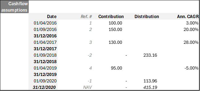
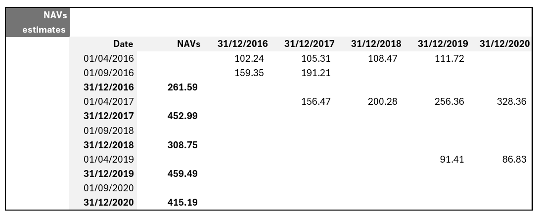
Assuming the investments’ growth over time is consistent with the Annualized CAGR above, using a standard [Investment*(1+CAGR)^time] formula, we can estimate the year-end Net Asset Value of the portfolio for the observed sub-periods (granular data per column, total in the NAVs column).

The historical problem of returns is aggregation. Unfortunately, averaging CAGRs that refer to different investment-divestment time horizons doesn’t work. The weighted average of CAGRs for the four investments is 13.61%. The implication is that the 475 invested over the 4 years and 8 months of the example would imply 871.19 [= 475*(1+13.61%)^(Dec. 2020 – Apr 2016/365)] of total portfolio value. But this outcome is nowhere near 761.62, which is the sum of distributions and final NAV.

This shortcut implies that all invested capital stays perpetually invested at the average CAGR, which replicates the reinvestment assumption that biases IRR. In other words, the fact that distributions do not earn their original CAGRs, or that later contributions do not yet earn their expected CAGRs, is lost in the calculations.

Unsurprisingly, the Internal Rate of Return (in its XIRR version, to take actual dates into account) produces a similar outcome, albeit amplified by the relatively quick but large first distribution (positive sign, with last NAV assumed as distributed).

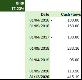
Neglecting duration, IRR is usually treated as a since-inception return, which implies that the 475 invested over the 4 years and 8 months of the example would produce 1,011.15 [= 475*(1+17.23%)^ Dec. 2020 – Apr 2016/365] of total portfolio value. This is clearly not the underlying economic reality of the analyzed PE portfolio.

It is worth remembering that a “proxy duration” concept, indirectly calculated by putting in IRR relative to TVPI, had been introduced[ii]^{, [iii]} but never properly exploited. That concept was also not designed to anchor performance measurement and compounding in a multiperiod perspective, with real-life time-weighting constraints, (i.e., the key conventions that tie the amounts of money due or received when an interest rate is attached to a mortgage or a swap). These conventions link a rate to a reference amount of money and a time horizon. They are the reasons why I ask anyone reporting returns if they would be able to pay that compounded return, for a given time horizon, if I provided the capital.

Also, the new NAV-to-NAV IRR approach neglects the importance of duration. It attempts to correct IRR flaws by calculating NAV-to-NAV Horizon IRRs, and then chaining them to approximate the growth of value over time, with a time-weighted logic. In the following chart, I have replicated the approach, first by calculating NAV-to-NAV IRRs (in other words, the XIRR for each calendar year, as shown in the Cash Flows and Horizon IRR sets of columns), then calculating inception-to-NAV and NAV-to-NAV compounded value multipliers (Horizon x column), and finally multiplying them to ultimately compute the annualized NAV-to-NAV return of 16.49% [=(1.07*1.17*1.23*1.15*1.16)^(365/Dec. 2020 – Apr 2016)-1].

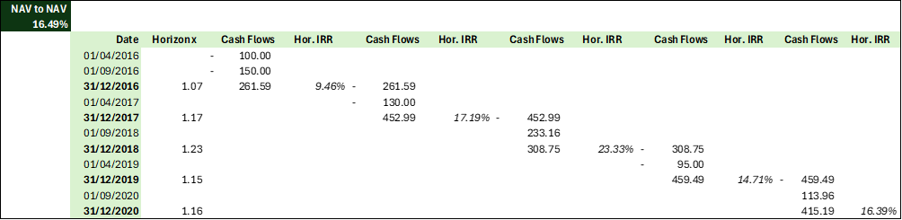
Compared to IRR, the NAV-to-NAV approach does not substantially improve the representativeness of the return calculated, compounded for the portfolio over its observed life: 981.44 [= 475*(1+16.49%)^ Dec. 2020 – Apr 2016/365]. It actually overestimates the total value produced by the portfolio by 28.75% over the observed period. It is worth mentioning that longer periods would amplify the difference because, in this approach, the implicit reinvestment assumption is also at work.

There is no way to reconcile time-weighted return and multiple cash flows transactions without a proper risk neutral utilization of duration. I have already illustrated the theory of the DARC approach in my prior article. Consequently, I would refer to the information provided there to illustrate how a proper two-cash flows synthetic transaction is constructed to represent the portfolio of this example.

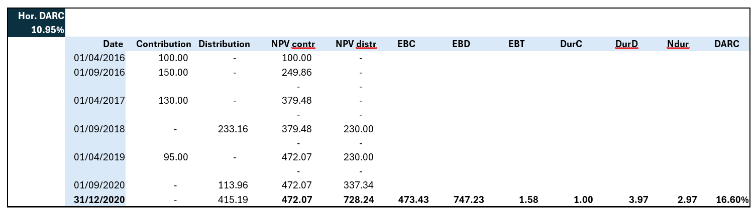
DARC is normally calculated on a daily basis for precision purposes. This procedure calculates the DARC as of the end of the observation period, on Dec. 31^st, 2020, with minor approximation. Given the actual rates on the USD risk free curve, the cumulative Net Present Value for both contributions and distributions are calculated. These amounts are then transferred over time to the natural forward placeholder of the durations of contributions and distributions (DurC and DurD). This forms the two bullet cash flows EBC and EBD, equivalent and not arbitrageable against the actual multi-cash flows portfolio. The EBT ratio between EBD and EBC allows the calculation of the annualized CAGR of the portfolio over its forward net duration Ndur, i.e. a DARC of 16.60%, over 2.97 years, 1.00 years forward.

DARC is a forward net duration return. It should not be automatically used as a since-inception measure. Firstly, it explains IRR in the context of time. Secondly, it can be recalculated as a spot yield, defined by its risk neutral, fully diluted DARC equivalent measure (calculated by annualizing the ratio EBD/NPV contr, over the 4.75 years of time horizon) of 10.95%.

The DARC duration approach delivers exactly the value of the cash flows given the risk free curve – in this example with a 1.45% approximation, due to the simplifications: 773.49 [= 472.07*(1+10.95%)^ Dec. 2020 – Apr 2016/365].

With this, it should be clear that it takes a full time-horizon, like a 10-year LP agreement, to extract the forward net duration return (that the IRR approximates and the DARC details).  Consequently, it should also be clear that IRRs cannot be compounded, neither in a since-inception nor a horizon perspective. Only DARC can be transformed to be compounded without losing representativeness of the underlying investment reality – always represented by the actual money invested and received, not by assumptions.
 

About the Contributor
 

Massimiliano Saccone is the Founder and CEO of XTAL Strategies and developed its patented DARC methodology. Beforehand, he was a Managing Director, ultimately Global Head of Multi-Alternatives Strategies, at AIG Investments, after stints at DWS, Deloitte, and KPMG. A CFA charterholder, qualified accountant, and auditor, he holds a Master's in International Finance from the University of Pavia, and a magna cum laude Master's in Business and Economics from La Sapienza University in Rome. He is an active volunteer at the CFA Institute, and a Lieutenant of the Reserve of the Guardia di Finanza.
 

Learn more about CAIA Association and how to become part of a professional network that is shaping the future of investing, by visiting https://caia.org/