


By Benn Eifert, Managing Partner and CIO and Scott Maidel, Head of Business Development at QVR.
This note discusses the role that tail hedging plays in a long-term asset allocation. Its focus is on the counterintuitive insight that hedging strategies with negative long-term expected return, when added into an asset allocation framework that is rebalanced regularly, can result in higher long-term compound rates of return.
This is not a novel insight, but in our experience, it is an extremely underappreciated point. It is particularly important in the current market environment:
- Near-Zero Rates: Looking forward, we are in a near-zero long term interest rate world.
- Limited Diversification from Fixed Income: It is unclear from here how much cushion fixed income can provide in a typical diversified portfolio.
- Erratic Behavior in Tail Events: We’ve seen erratic behavior amongst many asset classes and strategies that historically have been viewed as diversifying.
Given these dynamics, it is particularly important for long-term-focused assets owners to consider alternative sources of diversification, absolute return, and dedicated long convexity exposure.
Volatility and Drawdowns Decrease Long-Term Compound Returns
One popular argument goes as follows: “We are long-term investors. Volatility doesn’t matter to our portfolio.” This is an appealing idea. However, there are two main issues here.
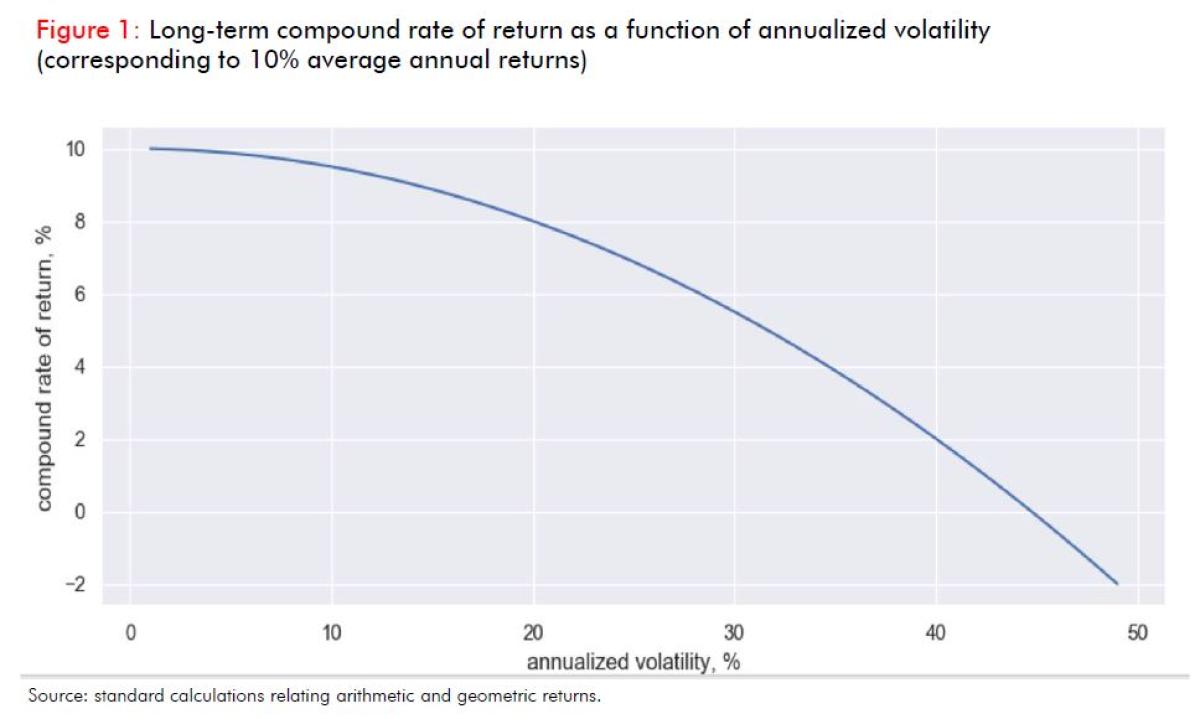
Variance Drag: Second, volatility itself reduces the long-term compound rate of growth of a portfolio, via a phenomenon called variance drag. Let’s consider two return streams, both with average annual returns of 10%, but with annualized volatility of 10% and 20% respectively. The long-term compound growth rates of the two portfolios will be 9.5% and 8.0%! The adjustment factor is equal to half of the variance (or squared volatility). A reduction in volatility from 20% to 10% for the same average annual return increases the long-term compound rate of growth by 150 basis points.
For sufficiently high volatility levels, a return stream with 10% average annual returns actually compounds at a negative long-term growth rate!
Simple Example: Start with $1 billion of equities and suffer a 20% drawdown, the equity exposure falls to $800 million. If equities turn around and rally 20%, the portfolio will make only $160 million, not the full $200 million you lost. This is the negative impact of volatility and drawdowns on the compound growth of a portfolio.
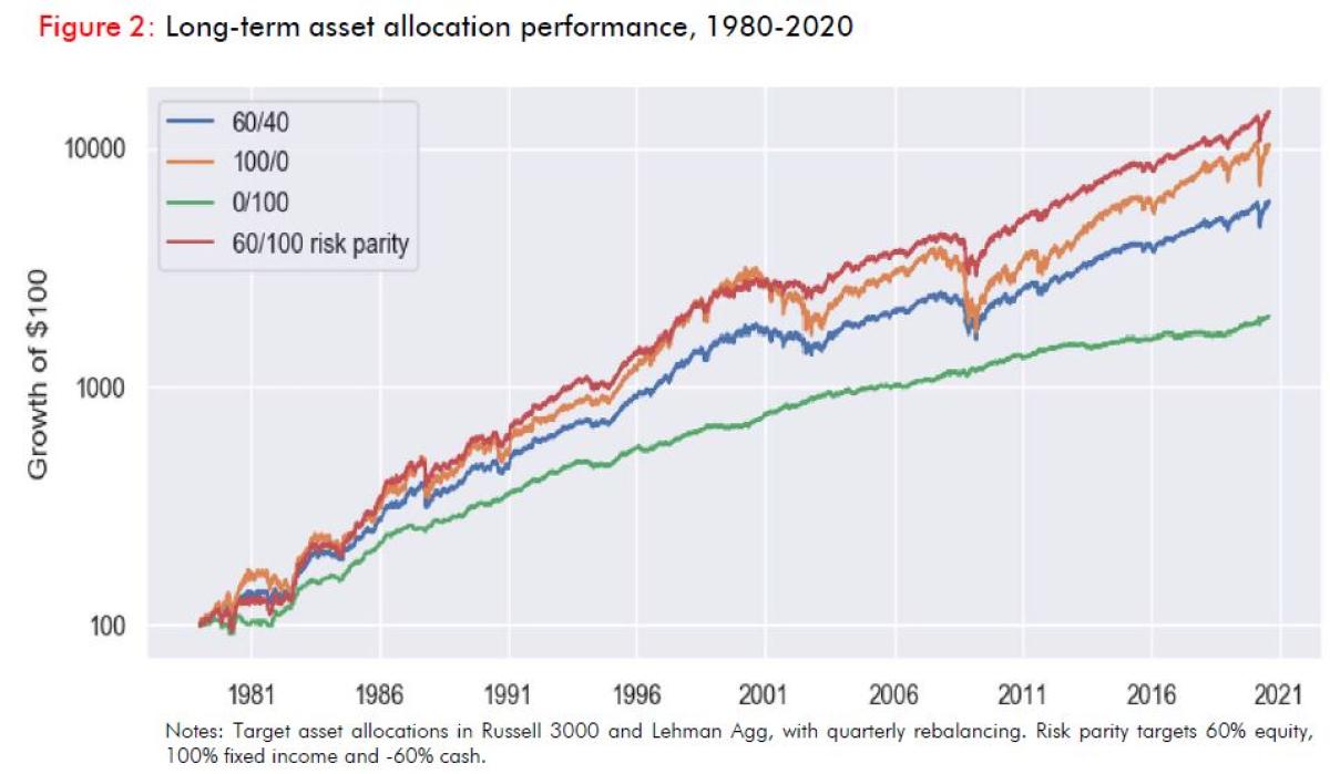
This has been one of the major motivating factors for the 60/40 portfolio over the last several decades. A long-term diversified asset allocation across equities and fixed income has benefited tremendously from the fall in interest rates since the 1980s. While equity returns have outstripped fixed income returns, fixed income has rallied sharply during most equity market selloffs, cushioning drawdowns and improving compound returns over time. Risk Parity strategies explicitly leverage this dynamic and have outperformed 100% equity allocations even in the post-2008 period of low interest rates (Figure 2).
Inverse Stock/Bond Correlation: This has become a core part of the assumptions behind portfolio construction. Under some regimes, it is reasonable to think that correlation can remain negative even at low levels of yields. For example, if the world remains mired in slow growth and low interest rates, rates will still likely drift mildly higher during more optimistic times and fall sharply during crises as central banks enact stronger and stronger countercyclical policy.
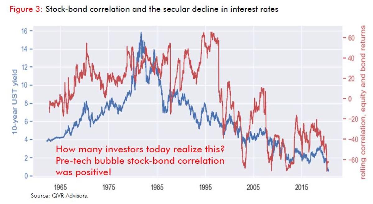
- Relatively New Phenomenon: However, inverse stock/bond correlation is a relatively new phenomenon historically and has tended to move back towards positive when central banks begin tightening monetary policy (see Figure 3).
- Correlation Breakdown: There are regimes where that correlation may well break down, especially if inflation starts to firm. A breakdown of inverse stock/bond correlation witnessed over the last 20 years, represents one of the greatest risks for a typical diversified asset allocation.
Tail Hedging Can Increase Long-Term Compound Returns
Another popular argument goes as follows: “Tail hedging involves buying various forms of option-based insurance against market drawdowns. Because markets generally charge a risk premium for insurance, the expected returns of a tail hedging strategy over long periods of time are negative. As a result, a long-term-oriented asset owner should not allocate to hedging strategies, as they will detract from long-term compound returns.”
Like many popular arguments, this is partly correct. Over the long term, you should expect negative returns from tail hedging strategies. The market would be wildly inefficient otherwise. Individual long convexity trades at certain points in time may be mispriced, and smart, dynamic hedging strategies might be able to reduce the cost of carry over time, but it is unrealistically optimistic to think that tail risk hedges can make money systematically over time.
The Portfolio Effect
This popular argument misses a key point: the portfolio effect. Tail risk hedges are inversely correlated with the performance of risk assets and produce outsized returns during times of crisis. As a result, if tail risk hedges are added to a long-term, regularly rebalanced portfolio, they can cushion drawdowns and mitigate the mechanical reduction of risk asset exposure during times of stress. In doing so, they can enhance the long-term compound rate of return of the investment program, despite the hedges themselves losing money over long periods of time.
Some people find this counterintuitive at first. How can adding a money-losing strategy to a portfolio cause that portfolio to make more money over time? Intuitively, it is because the outsized performance of a tail hedge during large market drawdowns allows a regularly rebalanced portfolio to have more dollar exposure to risky assets in the periods immediately following those large market drawdowns.
Think back to the simple example above of the $1 billion equity portfolio that suffers a $200 million drawdown. If you additionally held a hedge that offsets $100 million of those losses, after rebalancing the hedge gains back into equity exposure, the 20% rally will gain you $180 million. That extra $20 million is returns on equity exposure, not on hedge exposure. However, it was the presence of the hedge in the first place that enabled you to hold the additional equity exposure after the market drawdown that generated the $20 million. This is why hedging strategies can potentially enhance long-term portfolio compound returns even if the dollar returns of the hedging strategies are negative.
A leading example of a low-bleed hedge is a 1-year 30-delta put, dynamically delta hedged, and rolled quarterly. An outright put has some asymmetric exposure to volatility, and also has some linear short market exposure (or delta). The delta-neutral put only has the former. If we are considering a tail hedge, we are interested in adding convexity to the portfolio, not in altering the target equity exposure in the portfolio, which can be done independently of option hedges. The tenor of one year provides exposure to spikes in implied volatility and risk aversion while reducing the rate of option decay relative to short term maturities.
Our point here is not about this exact systematic hedge. Results are broadly similar for a range of longer-term downside puts. Furthermore, we at QVR are strong believers that hedging programs should be dynamic and source relatively inexpensive convexity where it is available at a point in time. If you want to chat about how we think about value opportunities on the long volatility and hedging side, feel free to reach out. But here we are focusing on how convex hedges work within an asset allocation framework, and how their marginal impact within such a framework is potentially very different than their stand-alone characteristics.
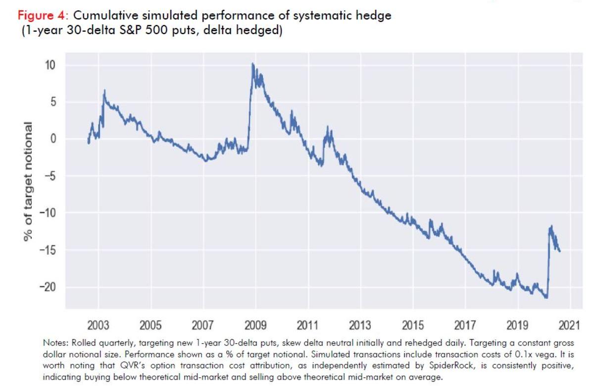
Our data here starts in 2002. As you can see in Figure 4, systematically buying 1-year 30-delta puts is a money losing proposition over the longer term. If we target a constant dollar notional size for our positions, rolling every quarter and delta hedging daily, our analysis indicates a cumulative loss of about 13% of that target notional size since 2002.
Importantly, note that these percentage returns are relative to notional, they are not returns on cash or capital. Option positions are highly cash efficient, with initial margin requirements of perhaps a few percentage points of notional on an appropriate prime brokerage platform.
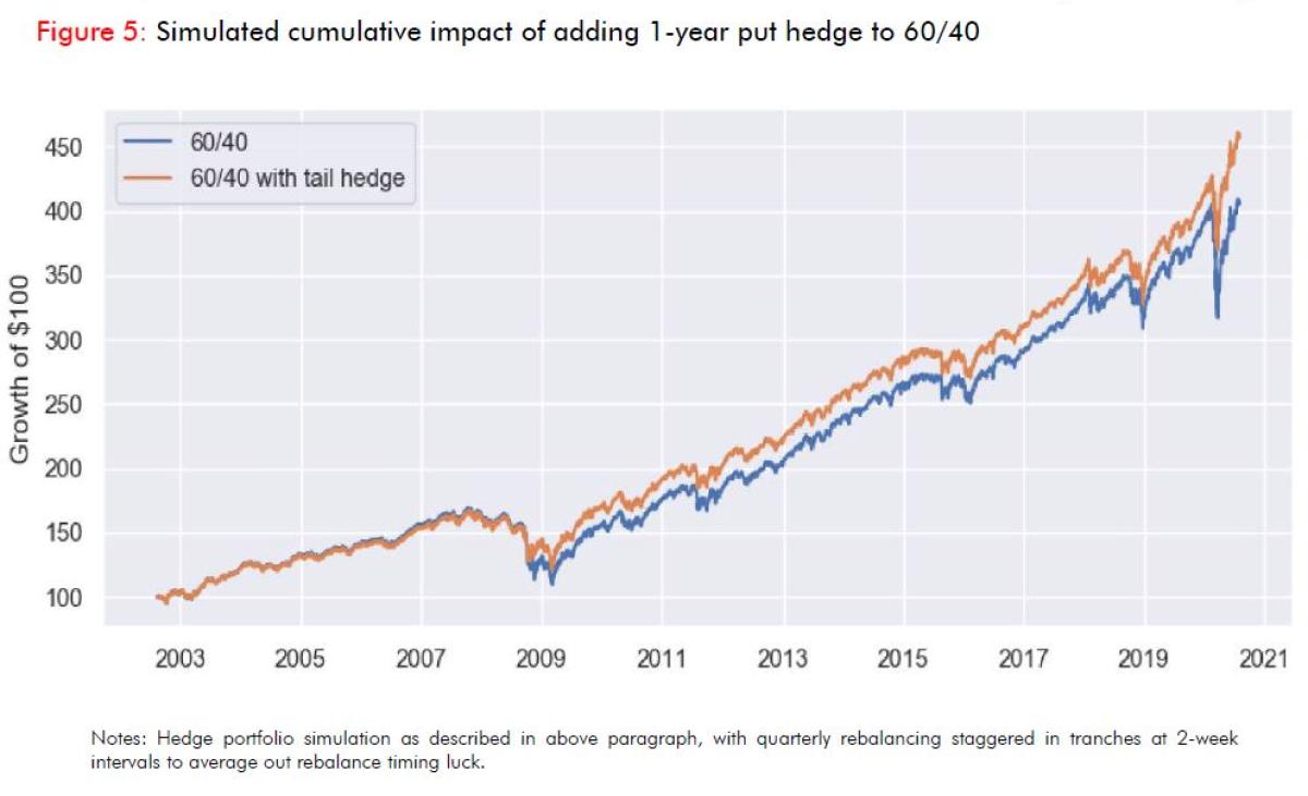
We simulate borrowing money to fund a constant-notional allocation to the tail hedge. We target an average investment in option premium equal to 1% of portfolio NAV, which ends up funding 25% of NAV in notional for the 1-year 30-delta put*. Keep in mind that option positions require only the premium to fund (not the notional).
We then rebalance the overall asset allocation quarterly, including the hedge. We implement the quarterly rebalance in tranches every two weeks, as if we had six sub-portfolios each with a quarterly rebalance at a different point in time. This smooths over rebalance timing luck, which is particularly important with convex and path dependent instruments like option hedges.
The orange line for the hedged 60/40 portfolio in Figure 5 unsurprisingly shows lower volatility and drawdowns than the unhedged portfolio.
However, importantly, note that:
- Total returns for the hedged portfolio are higher as well!
- The difference is a modest 25 basis points, with a compound growth rate of 8.04% vs 7.79%.
- But remember that we are adding a negative-long-term-return asset to the portfolio that is protective of the left tail (recall Figure 4)!
The point of this note is not to do a detailed analysis and comparison of many different systematic hedging strategies or rebalancing rules, but rather to illustrate the way that a hedge which has negative long-run expected returns but reduces drawdowns can actually be additive to long-run compound returns within an asset allocation framework.
That said, the basic results on that central point are not driven by the specific choices we’ve made here.
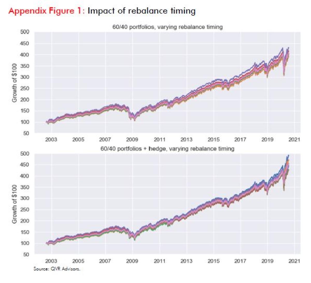
There is some real impact of rebalance timing when managing convex, path-dependent hedges (see Appendix Figure 1). We’re smoothing that out here by rebalancing incrementally in tranches, which generally we would recommend in practice. But even for the “concentrated” rebalances in Appendix Figure 1, the unlucky outcomes at the lower end of cumulative performance on hedged portfolios are as good as the lucky outcomes at the higher end of cumulative performance of the unhedged portfolios.
Also, there is nothing special about the 1-year 30-delta put, it is just a simple benchmark. You can vary this across a wide range of thematically similar structures that are medium to longer term with strikes skewed to the downside. Generally, our view is that the best risk/reward hedges change over time based on market conditions and flows. One should not over-focus on cherry picking structures that performed slightly better than others over the last two decades.
Institutional Realities: The Impact of Cutting Risk to Raise Cash Under Stress
Let’s next think about further long-term benefits of mitigating drawdowns. We hear statements like this quite often: “We aren’t thrilled with valuations here, but if we got a significant pullback in risky assets, we’d take the opportunity to add significantly.”
Many types of institutions which hold long-term oriented portfolios face challenges when dealing with large, sudden drawdowns.
- Spending Commitments: Pensions, foundations and endowments often have significant recurring spending commitments that need to be met.
- Capital Calls: They may have venture capital and private equity commitments which experience capital calls. They may have future spending plans that require preservation of capital at certain threshold levels.
- Organizational Realities: Or there may simply be organizational realities and psychology that amplifies risk aversion under stress.
As a result, erstwhile long-term-focused institutions often choose or are forced to sell risky assets and raise cash when their portfolios are experiencing large drawdowns.
Cutting market risk actively during drawdowns is one type of risk management, and it could hypothetically lead to averted losses in a protracted, trendy selloff. However, it leads to lower compound returns over the long run if risk assets have positive returns.
Figure 6 provides a simple example of the performance of a 60/40 asset allocation with quarterly rebalancing (blue line) over the period 1980-2020. The orange line provides a stylized example of the result if a 20% peak to trough drawdown induces a 20 percentage-point shift from equity into cash, which is moved back to 60/40 after half of the drawdown is recovered. This moves the compound rate of return from 10.32% per year to 9.97% per year over 1980-2020, a -37 basis points “negative convexity drag”. This arises because the risk-reduced portfolio misses the first leg of an asset market rebound.
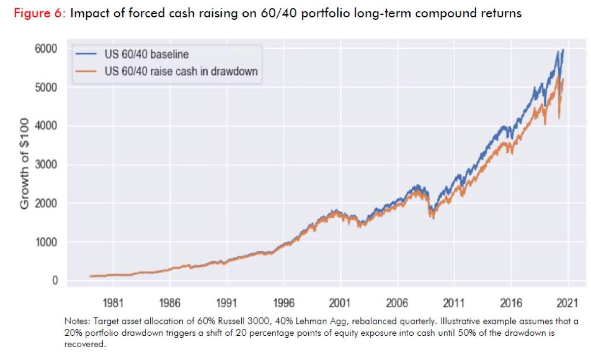
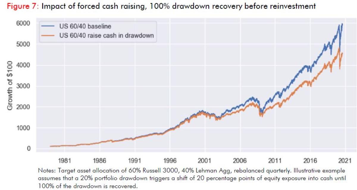
Figure 7 illustrates a similar exercise but where the asset allocation is only moved back to 60/40 after the full drawdown is recovered. This moves the compound rate of return down to 9.62% per year over 1980-2020, a -70 basis points drag relative to the standard 60/40.
These are just simple, stylized examples, and every organization is different in terms of the extent of internal pressures or needs to cut risk in a severe portfolio drawdown. However, we at QVR have seen many cases of this dynamic, including among very large institutions during the most recent market turmoil in March 2020. Recalling back to 2008-09, there were also many examples of large asset owners liquidating private equity and venture capital funds in the secondary market to raise cash. It is important to recognize that every crisis environment is different, and many large institutions find themselves under pressure in ways they did not expect.
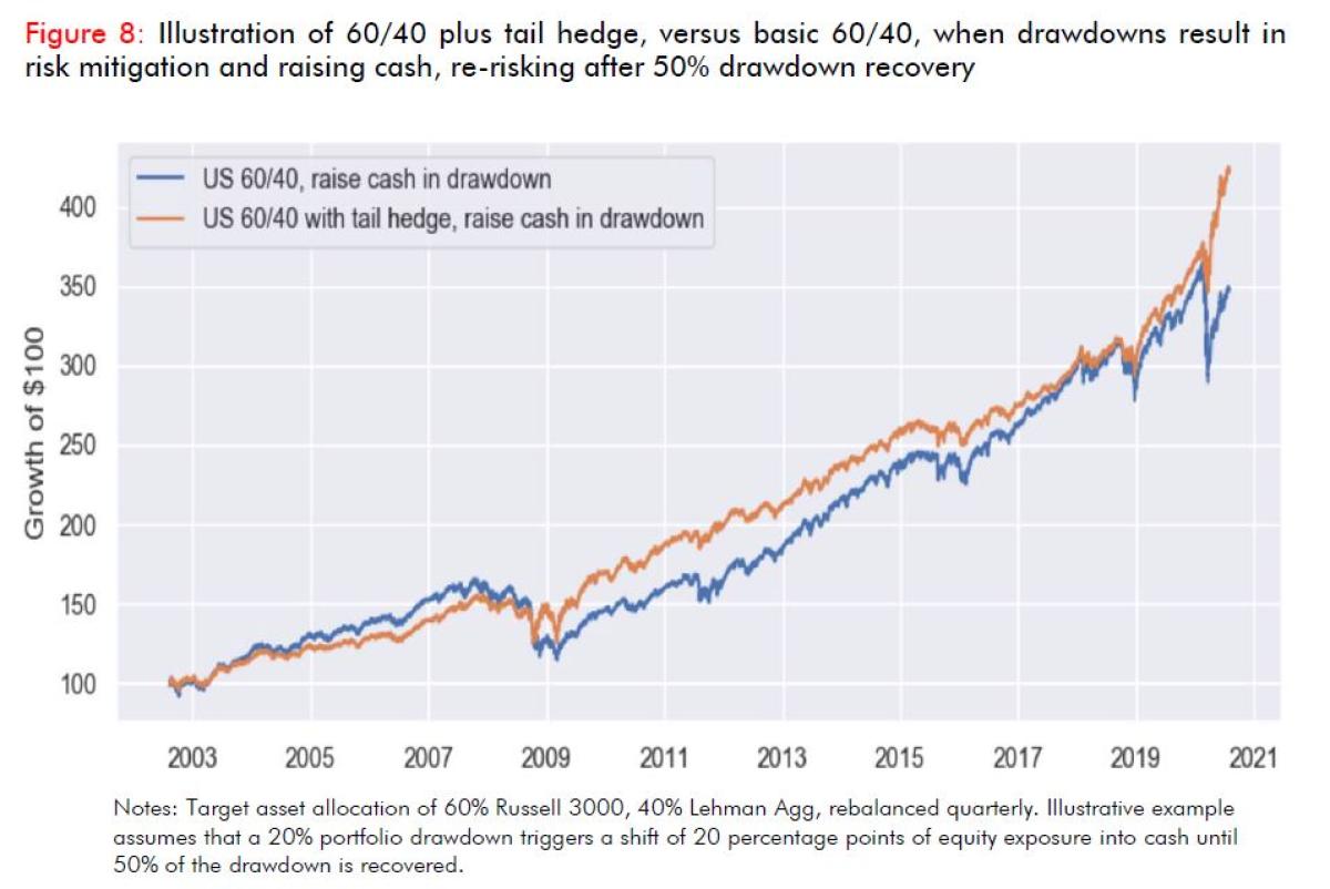
Let’s consider what happens if we add a systematic allocation to the same long-term strategic tail hedge from above, using the same methodology, rebalancing the entire asset allocation quarterly. As Figure 8 shows, the hedged portfolio has periods of underperformance and periods of outperformance, but the difference in compound rate of return is +105 basis points.
Is “Defensive Equity” a Better Substitute?
Another very common thing we hear, especially from consultants: “But options are systematically overpriced... instead of buying tail hedges, we prefer to overwrite calls or replace equity exposure with cash-secured puts in order to buffer downside risk and generate income.”
There are a few important issues raised here.
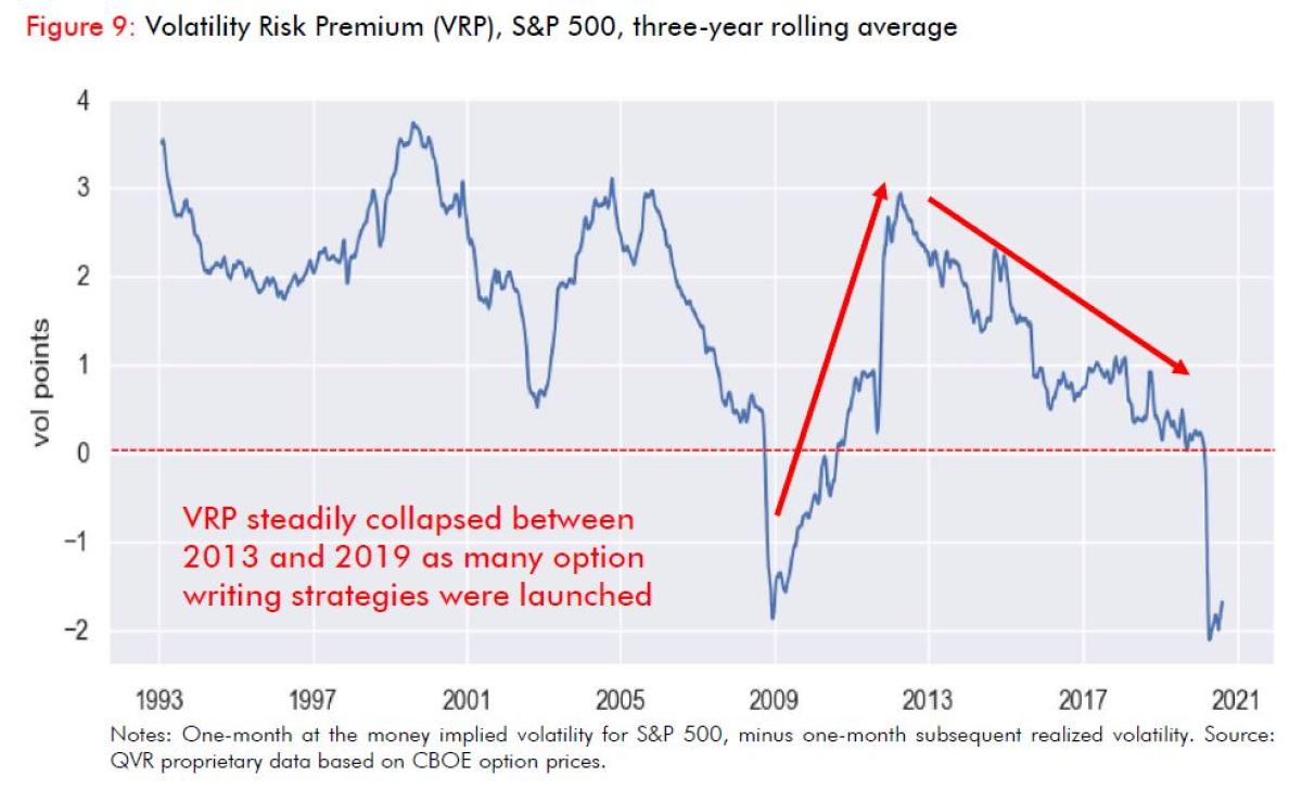
Volatility Risk Premium (“VRP”)?: First is the question of the risk premium associated with options. There is good evidence that short-term options were relatively expensive for many years. This is reflected in the observed volatility risk premium (1-month at the money implied volatility of S&P options, minus subsequent 1-month realized volatility). Figure 9 shows a trailing 3-year average. You can see how the volatility risk premium was high on average historically (2.5+ points on average) before the 2008 credit crisis. It recovered to high levels again after the crisis, before compressing dramatically again by 2019, to the point where there had been almost no risk premium on a trailing 3-year basis even before March 2020 crash.
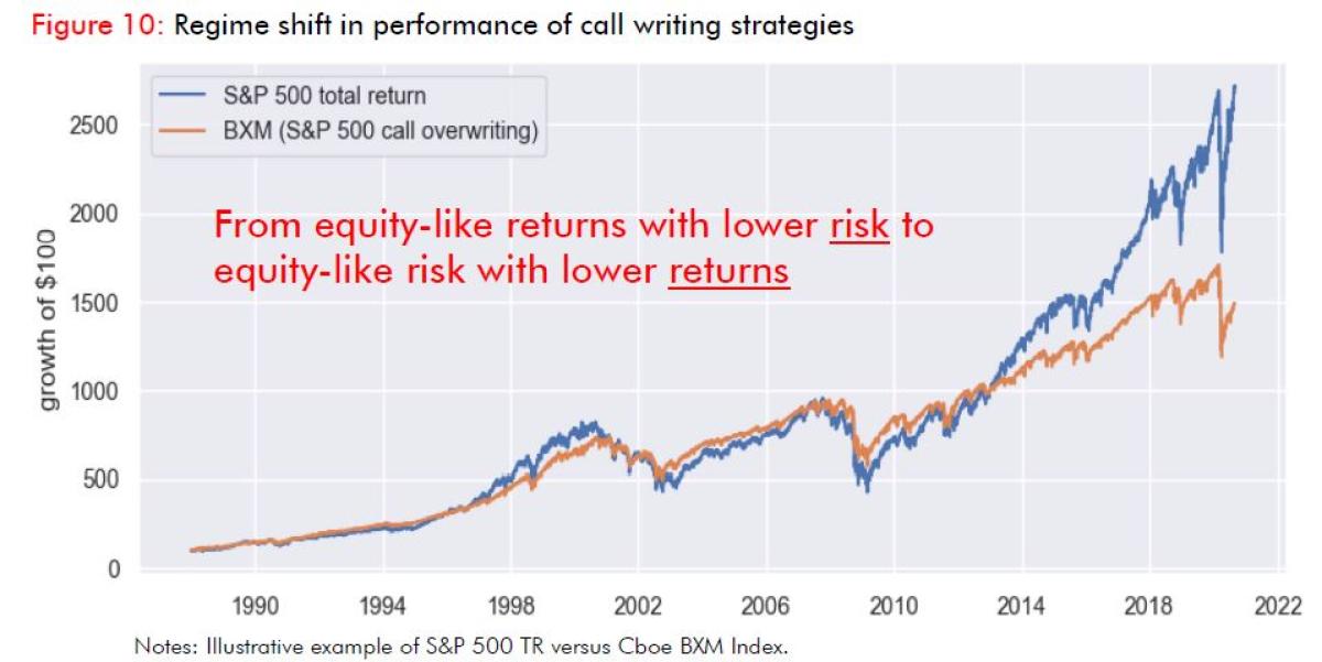
Regime Shift in VRP: This regime change in VRP is also reflected in the historical performance of the Cboe BXM (call overwriting benchmark) relative to equities (see Figure 10). For the period 1990-2013 one could characterize BXM as offering equity-like returns over the long term with reduced risk. However, this attracted very large inflows into short term option selling strategies, which had the mechanical effect of depressing short-term implied volatilities. Since 2013, one could more fairly characterize the Cboe BXM Index and PUT Index as offering equity-like risk with significantly lower returns.
Negative Convexity: Second, even holding a regime shift in VRP aside, we return to a central point of this note. Option selling strategies are negatively convex, so they usually experience disproportionate losses when other risky assets are down a lot. So even if they have made money in the long run, their marginal contribution to the long-term compound return of a rebalanced asset allocation may be smaller than the marginal contribution of an efficient tail risk hedging strategy, or negative.
Institutional Option Selling: A non-trivial part of that [option volume] growth has come from growing institutional participation in covered call and cash secured put write strategies in index, both the initial trades and then the recycling of that risk throughout the ecosystem. At its peaks in 2017 and 2019 we estimated the size of these programs at around $800 million vega sold per month. As we have discussed extensively in past letters, this flow has a steady dampening effect on volatility, because asset owners who sell short term options are effectively outsourcing aggressive daily equity portfolio rebalancing (buying dips and selling rallies) to dynamic hedgers of options positions. However, that dampening effect only exists near the strikes of the options being sold, which are typically short term (1 month) and near the money, so when markets push outside of their gravitational field, the coiled spring
can come loose.
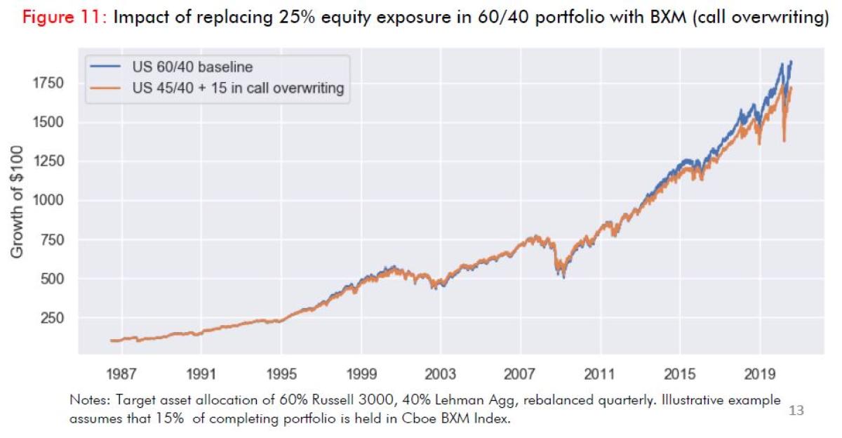
Where’s my Defensive Equity? Interestingly, large asset owners have been persuaded to join the short-term option selling party with path diversification and risk reduction arguments. However, Figure 4 [see similar Figure 10 and 11 here] illustrates what happens when global pension funds started viewing this niche derivatives strategy as part of their asset allocation around 2012-13. Over 2020's Q1-Q2, call write and put write benchmarks were down -15% and -12% respectively, versus -4% in the S&P. That scenario probably wasn’t in any of the pitchbooks for “defensive equity”.
Figure 11 shows the impact of replacing 15 percentage points of equity allocation with call overwriting over 1987-present. As expected, we see similar to slightly better risk-adjusted returns in the period prior to 2012, followed by steady underperformance of the allocation that includes call writing. Clearly there are no subtle diversification benefits embedded in call writing that cause an improvement in long-term asset performance despite the lower returns of call writing. Many investors have turned to option writing strategies to lower equity volatility. However, in the left tail a call overwriting strategy will behave much like a simple equity allocation. It is precisely the protection of the left tail that provides the variance drag reduction benefits that we need to improve for long-term compound returns.
That said, we at QVR strongly believe:
- Poor performance: Of short-term option selling strategies over the last 8 years stem from their incredible popularity and the large inflows into the space.
- Capped Upside: March volatility events caused large losses in such strategies, as they fell just as fast as equities on the downside but failed to capture the rebound nearly as well as equities.
- Re-evaluation: It is possible that we will see widespread re-evaluation of the role of these strategies in institutional portfolios, leading to rightsizing and a corresponding increase in risk premium.
Takeaways
- Exposure that are anti-correlated with risk assets in the left tail can enhance long-term compound returns of rebalanced asset allocations, even if they have negative returns on a stand-alone basis (tail hedges).
- A breakdown of inverse stock/bond correlation witnessed over the last 20 years represents one of the greatest risks for a typical diversified asset allocation.
- Many investors have turned to option writing strategies to lower equity volatility, but it is in the left tail that a call overwriting strategy will behave much like a cash equity allocation. It is precisely the protection of the left tail that provides the variance drag reduction benefits that we need to improve for long-term compound returns.
So, we reiterate, it strikes us that true long convexity exposure is particularly important for asset owners to consider as a part of their long-term asset allocation. Furthermore, given forward looking prospects for fixed income returns it is particularly important for assets owners to consider alternative sources of absolute return. Feel free to reach out if we can help you think through the implications for your investments.
Footnotes:
*Results are qualitatively similar for a constant-premium, varying-notional hedge, with the main difference being a larger hedge benefit in the March 2020 crash relative to
the October 2008 crash given the lower starting point of implied volatility in the former case.
About the Authors:
Benn Eifert was previously co-founder and co-portfolio manager of Mariner Coria, a relative value hedge fund on the Mariner Investment Group platform, which was seeded with $150 million by Alaska Permanent via the Mariner Incubation Fund. Before Coria, Benn was Head of Quantitative Research and Derivatives Trader for the Wells Fargo proprietary trading desk, which became the hedge fund Overland Advisors. Benn started his career as an emerging markets macroeconomist at the World Bank.

Benn has taught several classes in the Masters in Financial Engineering program in the Haas School of Business at UC Berkeley. Benn holds a PhD in Economics from UC Berkeley and BA in Economics and International Relations from Stanford University.
Scott Maidel joined QVR from Gladius Capital Management where he was most recently a Director of Institutional Solutions. He was previously Senior Portfolio Manager, Equity Derivatives at Russell Investments and Associate Director, Global Trading and Trade Research at First Quadrant. Scott has over 15 years of trading and portfolio management experience with global derivatives.

Scott holds a B.Sc. in Investments and Financial Markets from the University of Southern California, an MBA from Pepperdine University and is a Harvard Business School alumni of the Program for Leadership Development (PLD). Scott is a CFA charter holder and Financial Risk Manager (FRM) certified.
Disclaimer
The information contained herein is confidential and proprietary and provided for informational purposes only, and is not complete and does not contain certain material information about making investments in securities including important disclosures and risk factors. All securities transactions involve substantial risk of loss. Under no circumstances does the information in this document represent a recommendation to buy or sell stocks, limited partnership interests, or other investment instruments.
As with any investment, past performance is not necessarily indicative of future performance.
The information contained herein does not include certain information regarding investments in registered investment funds, alternative investment vehicles or hedge funds (each a “Fund” or collectively, the “Funds”), including important disclosures and risk factors associated with an investment in a Fund, and is subject to change without notice. If any offer is made to invest in a Fund, it shall be pursuant to a definitive Private Placement Memorandum prepared by or on behalf of the Fund which contains detailed information concerning the investment terms and the risks, fees and expenses associated with an investment in the Fund. Neither the Securities and Exchange Commission nor any state securities administrator has approved or disapproved, passed on, or endorsed, the merits of these securities.