


By Benn Eifert, Managing Partner and CIO, and Scott Maidel, Head of Business Development at QVR.
In the previous article, we made the case for considering tail hedging in a long-term asset allocation framework. In that original piece, we outlined how a tail hedge can potentially have a net positive impact on the long-term compound rate of return of an asset pool, despite that hedge line item losing money over time on its own. We contrast this with popular “defensive equity” approaches that involve option selling, which have detracted from long-term asset pool returns, because they are highly correlated with equities in market crashes, while tail hedges are highly inversely correlated.
Many people focus heavily on individual line items and are not used to thinking about portfolio interactions, finding this extremely counterintuitive.
We cannot count the number of times we’ve heard: “but hedges lose money over time, so a long-term-focused investor should never hedge.”
In this Common Hedging Discussions Part 2, we seek to debunk the myth associated with long-term, strategic tail hedging programs being detractors from long-term portfolio performance.
Figure 1 illustrates the historical simulated mid-market performance of a variety of simple rolling delta-neutral put hedges on the S&P 500. For each version, the options are rolled quarterly, targeting new options closest to the stated delta (20 or 30) and maturity (6 months to 2 years). Cumulative performance is shown as a % of target notional. The interpretation is (for example) that the simulated 6-month 30-delta rolling put strategy generated roughly 8% of notional in performance at peak during the 2020 pandemic crash, such that an equity portfolio protected 100% notionally would have experienced a 26% peak-to-trough drawdown instead of 34%.
Positions are dynamically delta hedged. This is important. The purpose of a tail hedge is to add convexity (large protective benefit in extreme market moves), not to reduce asset allocation targets for equity. Buying outright put options against an equity portfolio has the effect of lowering the effective equity allocation. A target 60% equity /40% fixed income portfolio where the equity exposure is notionally hedged with outright 30-delta puts will only have a 60% * (1 – 30%) = 42% equity exposure on rebalance dates. In contrast, a delta-neutral hedge overlay does not change average equity exposure. If an asset owner desires less equity exposure on average, they can just cut their equity target weights. The purpose of tail hedges is to allow asset owners to maintain equity exposure while reducing left tail risk and potentially improving long-term compound returns.
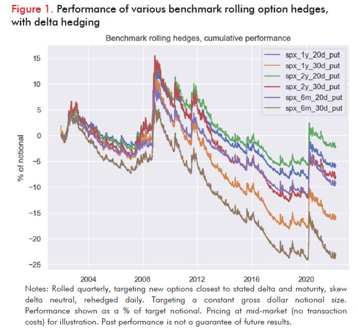
Importantly, note that all these simple rolling hedges lose money on average over the sample period, despite three large crises (the 2002 tech bust, the 2008 credit crisis, and the 2020 pandemic) along with a variety of moderate ones. This is expected. The purpose of the prior note was to remind the reader that the stand-alone returns of one component of a portfolio does not provide enough information to judge the contribution of that component to the
overall portfolio. In our experience, most people know this to be true conceptually, but significantly underestimate its importance in practice, and do not have good analytics for evaluating it.
ASSET ALLOCATION PERFORMANCE WITH ROLLING OPTION HEDGES
Now we apply the various benchmark rolling hedges above to a standard asset allocation exercise. This works as follows. We take a standard 60% equity (Russell 3000 Index) / 40% fixed income (Lehman Brothers Aggregate Bond Index) asset allocation. For the hedge overlay, we set the notional size target to 100% of equity exposure, and fund option premium at the risk-free rate (rather than reducing other exposures). This is slightly different from the analysis in our earlier note, which targeted option premium, because with a constant notional target it is easier to ensure comparability between a wide variety of different option hedge structures with different moneyness and tenor. We implement quarterly rebalancing of the asset allocation back to target weights. We do so on six different schedules spaced out by two weeks to mitigate rebalance timing luck.
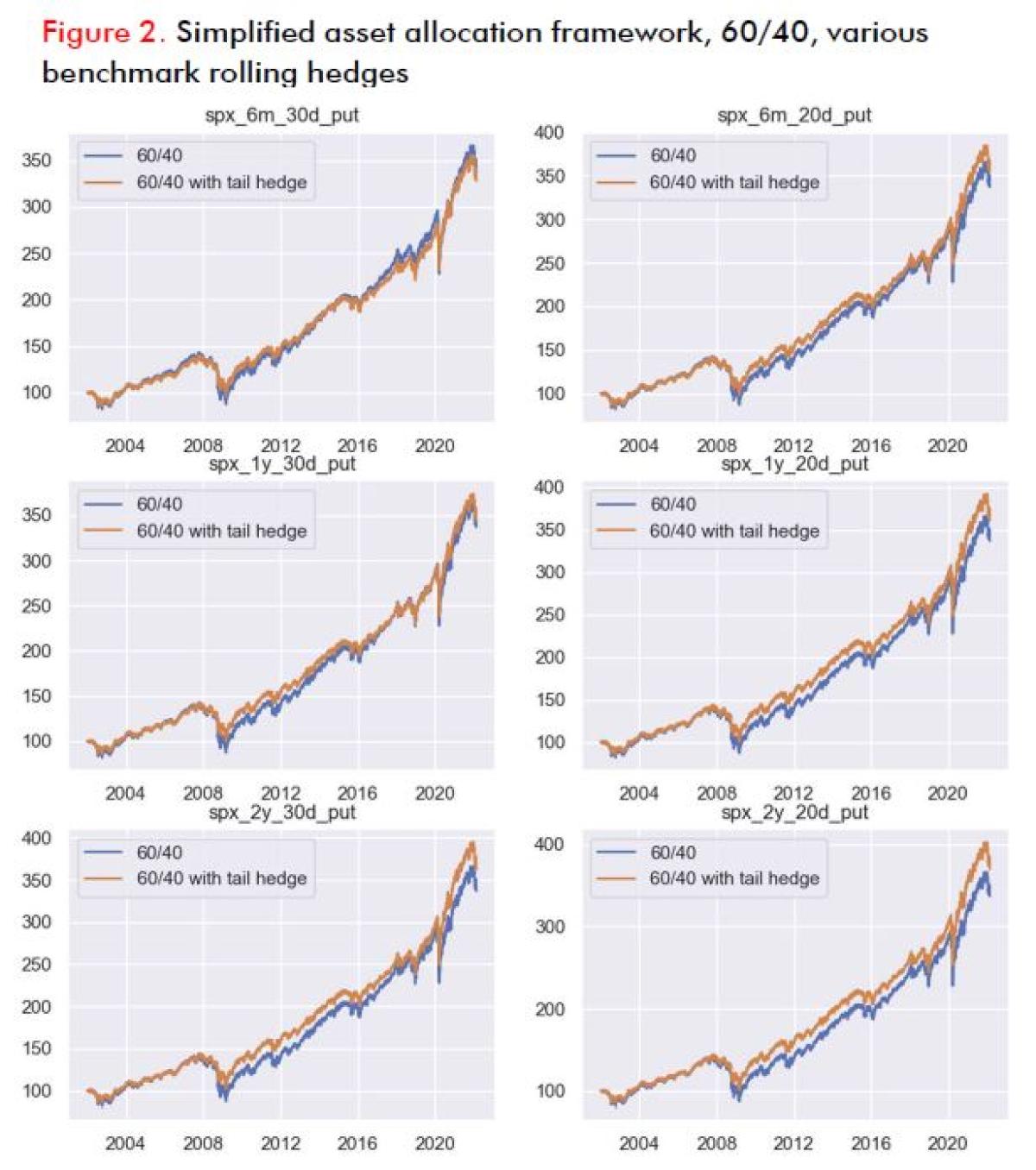
Notes: asset allocation with 60% weight on Russell 3000 Index and 40% weight on Lehman Brothers Aggregate Bond Index. Tail hedge overlays use the strategy indices described in Figure 2, with target notional equal to 100% of target equity exposure, and long option premium is financed at the risk-free rate. Quarterly rebalancing of the asset allocation back to target weights on six different two-week intervals (results averaged across rebalance schedules to mitigate rebalance timing luck). Pricing at mid-market (no transaction costs) for illustration. Past performance is not a guarantee of future results.
Figure 2 shows the results in terms of simulated growth of the NAV of the asset pool over time. Note how hedges sharply cut losses in 2008 and 2020, experiencing modest decay relative to unhedged 60/40 during long periods of quiet. As described in our Q3 2020 note, five out of the six simple benchmark hedges result in a higher simulated total portfolio return over the period, despite the hedges losing money on a stand-alone basis.
Table 1 summarizes these results. In terms of risk, clearly the hedged versions of the asset allocation are more stable, experiencing mid-9% annualized realized volatility versus 11% unhedged, and around 30% max drawdown versus almost 40% unhedged. This is not surprising and is the part that most hedging discussions focus on.
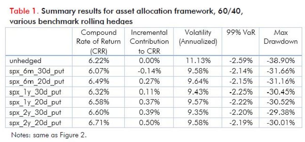
The more interesting thing is the differences in compound rate of return. The ICCRR (incremental contribution to compound rate of return) in the second column is the impact of each simple benchmark hedge on portfolio CRR. Five out of six ICCRR’s are positive, ranging from +0.11% basis points to +0.50%; only the 6-month 30-delta put is negative, at –0.14%. By adding a negative-performing line item to a rebalanced asset allocation, in these cases we are seeing higher simulated long-term rates of return from the overall asset allocation over the 2002-22, because that line item tends to be up big at the same time the core portfolio is down big.
The impact of tail hedges on an asset pool’s long-term compound rate of return depends on the weight of equity and equity-like risk assets in the portfolio. In the last few years, the forward-looking returns on fixed income exposures fell with low or negative real yields, rising inflation and prospective interest rate hikes. In response, many asset owners are cutting fixed income allocations in favor of larger private equity and venture capital exposures. Many large institutional portfolios are nowhere close to 60/40 anymore. The more equity-oriented an asset allocation is, the more powerful the portfolio benefits of hedges.
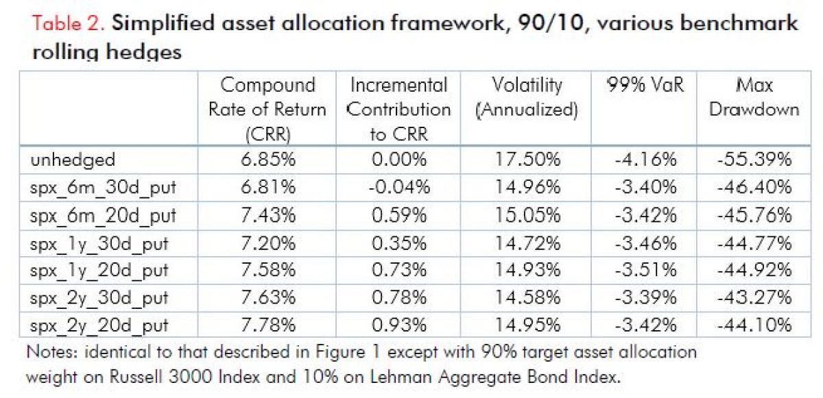
Table 2 illustrates the summary statistics for a more aggressive 90% equity, 10% fixed income asset allocation. Note that the unhedged compound rate of return for 90/10 is only modestly higher than 60/40 (6.85% vs 6.22%) with much larger max drawdowns (-55.4% versus -38.9%). The same dynamics are at work here; fixed income’s diversification benefits during crisis were quite strong over the past two decades.
Our six benchmark rolling hedges have significantly higher ICCRR for the 90/10 portfolio as compared to 60/40. Five out of the six have positive ICCRR, with the 6-month 30-delta put still negative but -0.04% versus -0.11% for 60/40, and the others ranging from +0.35% to +0.93%. The hedge benefits in most cases are roughly twice as large.
COMPARISON TO “DEFENSIVE EQUITY’ OPTION SELLING APPROACHES
Some common views among asset consultants is: “Option selling as equity replacement is a preferable alternative to hedging. Option selling is more efficient since call write and put write strategies have positive expected return over time but are less volatile than ordinary equity exposure.”
Or restated as: “Options are systematically overpriced, instead of buying tail hedges, we prefer to replace equity exposure with cash-secured puts or overwrite calls in order to buffer downside risk and generate income.”
Below we consider four common Cboe benchmark indices for option selling as equity replacement:
- BXM: call overwriting
- BXMD: out of the money call overwriting
- PUT: cash-secured put selling
- CNDR: iron condor (put spread and call spread) selling
The first two, BXM and BXMD, are long equity exposures with option selling overlays. BXM is the most popular S&P 500 call overwriting benchmark. BXMD is a variation on BXM where the options sold are out of the money 30-delta calls instead of near the money calls. PUT is a cash-secured put selling benchmark. CNDR is an iron condor selling strategy that sells call spreads and put spreads and is the only one of the four which is delta neutral on option roll dates, relying only on volatility risk premium and not on equity exposure to generate returns over time.
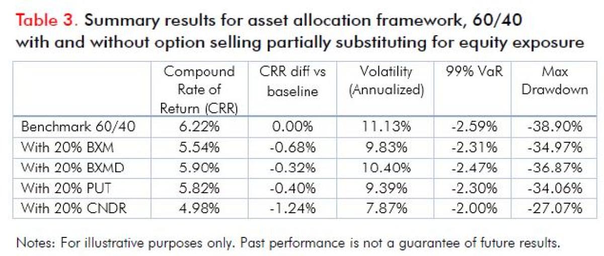
Figure 3/Table 3 illustrates how performance for the 60/40 asset allocation compares to versions which substitute a third (20 percentage points) of their ordinary equity exposure for option selling. Long-term returns are lower across the board. Risk metrics are lower, as the proponents of these strategies suggest, with max drawdowns down from 39% to the 27-35% range. Particularly during 2008 these benefits were evident as option selling performed relatively well during the protracted drawdown and steady recovery. However, the long-term CRRs are materially lower than the benchmark 60/40, ranging from –0.32% to –0.68% for versions including call and put write to –1.24% for the version including iron condor selling.
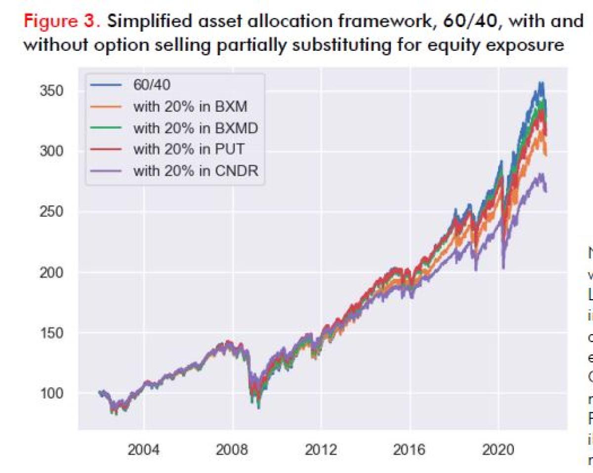
Notes: benchmark (blue line) is asset allocation with 60% weight on Russell 3000 Index and 40% weight on Lehman Brothers Aggregate Bond Index. Then we individually recalculate the performance of the asset allocation substituting 20 percentage points of equity exposure for option selling programs represented by the Cboe BXM, BXMD, PUT and CNDR indexes. Quarterly rebalancing of the asset allocation back to target weights. Pricing at mid-market (no transaction costs) for illustration. Past performance is not a guarantee of future results.
These results are as expected and the asset consultants who promote defensive equity strategies would say that the lower returns are an intentional tradeoff against risk reduction. However, volatility selling strategies as equity replacement offer some path diversification, but not outright risk reduction in all types of paths. An option selling strategy is not inherently risk-reducing: a cash-secured put selling strategy has the same exposure as outright equities in a sharp market selloff. Option selling strategies are short convexity (loses money at a faster rate the worse things get), not long convexity like a tail hedge. As a result, while they may make money over time on a standalone basis, they are potentially less additive from an overall portfolio perspective to an already equity-heavy asset allocation.
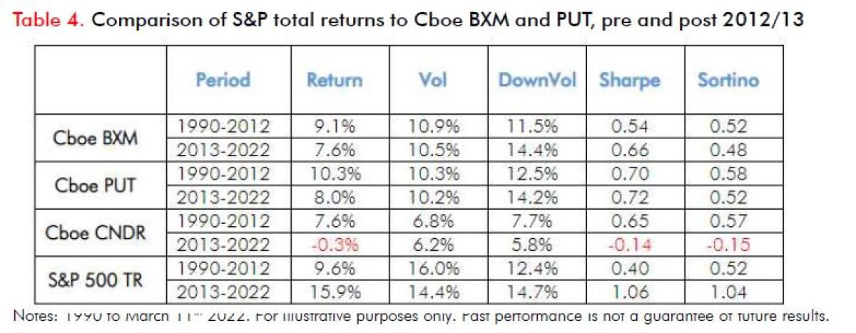
There are market environments in which option selling strategies have historically generated equity-like returns or better with lower volatility and downside capture. When option flows from end users are skewed to buy and risk premiums are high, such as 2001-05 and 2009-12, this is apparent.
As shown in Table 4, during 2013-20 when option selling strategies were very popular, and markets tended to crash quickly on high volatility and bounce back quickly, returns in option selling strategies fell dramatically relative to simple equity exposure. The potential risk reduction benefits from option selling strategies as equity replacement come in a slower selloff where elevated risk premium captured over time helps to materially offset losses on exposure. We discuss this and a lot more in our 2021 paper, Common VRP Discussions.
REBALANCING AND MONETIZATION
All the results above depend importantly on regular rebalancing as part of asset allocation and portfolio construction. That means regularly replenishing hedge budgets during normal market conditions and then steadily monetizing hedges during periods of extreme market stress.
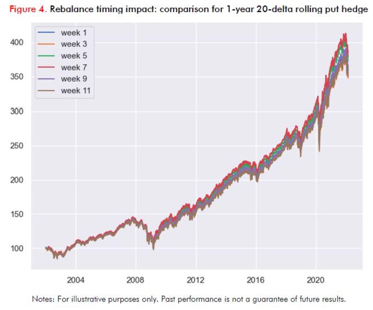
There are various approaches to this. The simple assumptions used for our analysis are purely calendar driven, with quarterly rebalancing of the entire asset allocation back to target weights. This raises the quantitatively important issue of rebalance timing luck, especially given the possibility of rapid crises and recoveries like March 2020. One rebalancing calendar might miss most of a large market drawdown and a volatility spike and only rebalance after the rebound; another might rebalance right at the bottom. Figure 4 illustrates the impact of rebalance timing luck over a long horizon, with quarterly rebalancing on six different cycles offset by two-week increments. Our results shown above average across these cycles, effectively assuming small partial rebalances regularly. This may not be practical for a large asset owner across their whole portfolio but can be approximately implemented via overlays.
For tail hedges specifically, it may make sense to have explicit rebalancing or monetization triggers based on market moves and not just the passage of time. The key here is in striking the right balance between the desire to capture gains and the need to deliver outsized performance in times of crisis. Tail hedges are by nature highly convex, providing much more incremental benefit when equities fall to – 30% below the highs from –20% below versus when they fall the first 10% from the highs. And the contribution of tail hedges to long-term portfolio performance comes from delivering outsized gains when core portfolios are getting wrecked. So, selling those hedges too early is self-defeating.
Figure 5 illustrates this by plotting the cumulative performance of a rolling 3-month variance swap position on the S&P 500 through 1H 2020 along with various exit triggers that might have been struck based on historical performance during previous market stress events.
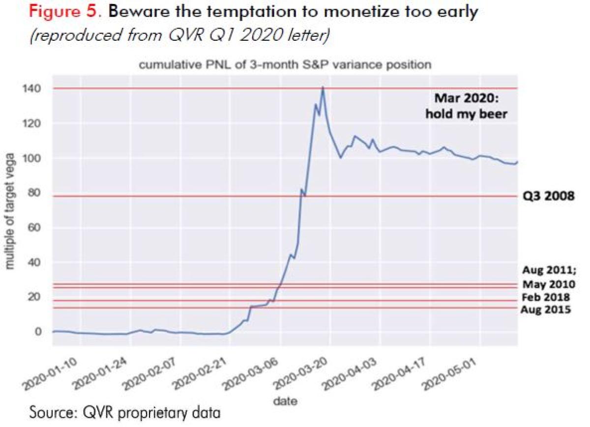
We often relate the story of the largest participant in the VIX options complex, an asset manager that volatility traders termed 50 Cent because of its hedging strategy of buying front month VIX calls targeting the contracts with a price around $0.50. That asset manager had experienced several smaller stress events like February 2018 where its VIX calls performed very well briefly but retraced all its gains. During late February and early March 2020, they aggressively liquidated their hedge portfolio for a decent gain, with the front month futures (the underlying for their call options) trading in the 25-30 range. Two weeks later those futures hit 80+. The hedging program made a small fraction of what it could have at peak. Meanwhile, the scale of the selling pressure was pushing the underlying March 2020 VIX futures below theoretical arbitrage boundaries with respect to the S&P 500 volatility surface.
Three points here:
- Market-conditions-based monetization strategies should be incremental based on a ladder of triggers, rather than binary. There is no set of data points that are reliably predictive of the scale of a selloff or how much further it could go that gives an asset owner high confidence in what is to come. Avoid over-fitting mental models to inherently small samples of historical crises.
- Monetization strategies should be simple enough to track easily but also price dependent. There are scenarios in which markets are very stressed, but option prices have not risen enough to be very expensive relative to extreme realized volatility. In such cases, simply buying synthetic equity exposure against tail hedges may be the best decision. Keep in mind the story of 50 Cent; know if the thing that you own and are trying to sell is extraordinarily cheap (possibly because you’re trying to sell so much of it into a dislocated market!). In other cases, option prices may have risen very excessively relative to the equity market selloff, and it is better to sell the core hedge positions. 2011-12 was a great example of this with the extreme bid for long-term equity index volatility.
- Ideally, monetization strategies should be framed in advance to coordinate expectations and mitigate behavioral biases. That does not mean they have to be mechanical – every crisis is different, and a large asset owner may find themselves putting on large opportunistic trades in very dislocated markets and wanting to keep more of their hedges than the otherwise would. But managers and clients should be on the same page about the expected approach to monetization and triggers set out in advance should raise decision points. Otherwise, it is too easy to act like a deer gazing into headlights.
STRATEGIC OWNERSHIP
Tail hedging programs most commonly fail because an organization is unable to view the asset allocation as a whole. When an individual portfolio manager is delegated ownership of the hedge line item, and the organization focuses on the stand-alone performance of the hedge line item as if it is an ordinary fund investment, this inevitably leads to hedge fatigue and to poor decision making around rebalancing and monetization. Organizations that are able to effectively deploy tail hedging programs have buy-in at the very top, and the tail hedging program should be viewed in conjunction with the asset base it is hedging. In such organizations, the asset allocation and portfolio construction function owns hedging and rebalancing, and they utilize analytics for attributing the portfolio-level benefits on both a realized basis and a simulated what-if stress scenario basis, offering deep-dive educational sessions to boards and other people in governance positions.
TAKEAWAYS
- If an asset owner desires less equity exposure on average, they can just cut their equity target weights. The purpose of tail hedges is to allow asset owners to maintain equity exposure while reducing left tail risk and potentially improving long-term compound returns.
- The stand-alone returns of one component of a portfolio does not provide enough information to judge the contribution of that component to the overall portfolio.
- Typically, we see higher simulated total portfolio return over any given period, despite the hedges losing money on a stand-alone basis.
- The ICCRR (incremental contribution to compound rate of return) is the impact of each simple benchmark hedge on portfolio CRR.
- Tail hedging program should be viewed in conjunction with the asset base it is hedging.
Check out their webinar on Managing Volatility Amid Heightened Inflation
Footnotes:
1. In particular, positions are hedged skew delta neutral (or “floating strike delta neutral”). Given that the S&P 500 implied volatility surface is always downward sloping as a function of strike within the relevant range, this means a smaller amount of delta bought against a put, as compared to Black-Scholes. Delta-neutral put options hedged on a Black-Scholes delta would have a higher positive drift than Figure 1 and would experience smaller gains in market selloffs.
APPENDIX
About the Authors:
Benn Eifert was previously co-founder and co-portfolio manager of Mariner Coria, a relative value hedge fund on the Mariner Investment Group platform, which was seeded with $150 million by Alaska Permanent via the Mariner Incubation Fund. Before Coria, Benn was Head of Quantitative Research and Derivatives Trader for the Wells Fargo proprietary trading desk, which became the hedge fund Overland Advisors. Benn started his career as an emerging markets macroeconomist at the World Bank.

Benn has taught several classes in the Masters in Financial Engineering program in the Haas School of Business at UC Berkeley. Benn holds a PhD in Economics from UC Berkeley and BA in Economics and International Relations from Stanford University.
Scott Maidel joined QVR from Gladius Capital Management where he was most recently a Director of Institutional Solutions. He was previously Senior Portfolio Manager, Equity Derivatives at Russell Investments and Associate Director, Global Trading and Trade Research at First Quadrant. Scott has over 15 years of trading and portfolio management experience with global derivatives.

Scott holds a B.Sc. in Investments and Financial Markets from the University of Southern California, an MBA from Pepperdine University and is a Harvard Business School alumni of the Program for Leadership Development (PLD). Scott is a CFA charter holder and Financial Risk Manager (FRM) certified.
Disclaimer
The information contained herein is confidential and proprietary and provided for informational purposes only, and is not complete and does not contain certain material information about making investments in securities including important disclosures and risk factors. All securities transactions involve substantial risk of loss. Under no circumstances does the information in this document represent a recommendation to buy or sell stocks, limited partnership interests, or other investment instruments.
As with any investment, past performance is not necessarily indicative of future performance.
The information contained herein does not include certain information regarding investments in registered investment funds, alternative investment vehicles or hedge funds (each a “Fund” or collectively, the “Funds”), including important disclosures and risk factors associated with an investment in a Fund, and is subject to change without notice. If any offer is made to invest in a Fund, it shall be pursuant to a definitive Private Placement Memorandum prepared by or on behalf of the Fund which contains detailed information concerning the investment terms and the risks, fees and expenses associated with an investment in the Fund. Neither the Securities and Exchange Commission nor any state securities administrator has approved or disapproved, passed on, or endorsed, the merits of these securities.