

By Andrew B. Weisman, Managing Partner and Chief Investment Strategist at Windham Capital Management.
Introduction:
What is monetary policy, how is it conducted and what can we expect going forward? Presented below is a brief primer on the topic.
Monetary policy in the US is somewhat narrowly understood to consist of setting short-term interest rates as part of a thoughtful process that accommodates both a desired rate of inflation and a desired pace of economic activity. Of course, there is a great deal more to a central bank’s tool kit than the setting of interest rates, notably the management of its own portfolio of securities, or as it’s referred to in the US the “System Open Market Account,” but for the purposes of this discussion I limit myself to interest rate policy.
The Taylor Rule:
In 1993, the conduct of monetary policy was normatively conceptualized in a simple equation known as the Taylor Rule. Stanford economist John Taylor proposed the Taylor rule in a paper that was published in the Carnegie-Rochester Conference Series on Public Policy.[1] The rule was designed to provide a simple, transparent, and logical guide to help central banks determine the appropriate level of short-term interest rates to achieve their macroeconomic objectives. The interest rate typically referenced in the United States as our central bank’s (the Federal Reserve, or simply “the Fed”) key policy rate is the Federal Funds rate, or Fed Funds rate. The Fed Funds rate is the interest rate that banks and other depository institutions lend money to each other overnight; typically done to meet reserve requirements set by the Fed. A reserve requirement is the amount of money that banks and other depository institutions are required to hold in reserve, either as cash or on deposit with the Federal Reserve, as a percentage of their deposits (the money they take in from you and me). Think of these reserves as money that is kept available to return to you and me, should we request it.
A basic specification for the Taylor rule equation is presented below: Don’t look at the equation if it unsettles you as I restate it in layman’s terms below.
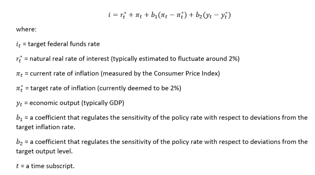
What this equation says is that central banks should set interest rates in response to: a natural real rate of interest (explained in more detail below), deviations from a desired rate of inflation, and deviations from a desired rate of economic growth.
The Taylor Rule implies that when inflation rises above the Fed’s inflation-rate target or when the economy is growing faster than its long-term potential, the Fed should raise the Fed Funds rate. Conversely, when inflation falls below target or when the economy is growing slower than its long-term potential, the Fed should lower the Fed Funds rate.
From a practical standpoint, the Taylor Rule presents several challenges for policymakers. First, much of the required data is either unavailable on a timely basis or simply unknowable, and second, the coefficients of the equation are somewhat arbitrary; just how strongly should a policymaker react to deviations from desired outcomes?
Let’s consider the first term in the equation, r*. This variable is a theoretical equilibrium “real” interest rate (an actual or “nominal” interest rate minus some measure of inflation) that is consistent with the economy being at full employment while maintaining low stable inflation, in the long run. r* has been variously estimated to fluctuate around 2% per annum.[2]
This interest rate is not, however, directly observable, rather it is estimated. One of the most common models used to estimate this variable is the Laubach-Williams model, which was developed by two Federal Reserve economists, Thomas Laubach and John Williams. This econometric (mathematical) model incorporates measures of economic growth and inflation while employing the Keynesian[3] notion that real interest rates are inversely related to consumption and investment. To make a potentially long story short, this component of the Taylor rule (r*) is not directly observable and can only be estimated with a considerable lag. Additionally, depending on the model you use, you’ll get a potentially very different number.
Now let’s consider π, inflation. It is worth noting that inflation is a rate, not a level. It represents the percent change in prices over a proscribed time interval. Inflation is typically reported on an annualized basis. However, depending on the time interval you’ve chosen, the resulting number can vary dramatically. This year in particular, inflation readings are highly subject to interpretation as the bulk of the variability in inflation data that we are currently observing, is being driven not by what is happening now to prices, but rather, by what is being dropped out of the calculation from the prior year as we step forward in time. This is the so-called “base effect.” For example, if inflation moved up this month but you drop out an even bigger month from a year ago, then your annualized measure of inflation will actually decline. So, what is inflation? Well, this year, depending on the starting date of your measurement period, the numbers vary from positive to negative. Currently, if you look back 12 months then we have considerable inflation. If you look back 4 months, we have deflation!
Finally, let’s consider y, economic output, which is typically proxied by the percent change is Gross Domestic Product (GDP), a broad measure of all consumption spending, government spending, investment spending, plus the value of all exports minus imports. Make no mistake, this is an enormous data collection project. So much so, that GDP is produced only quarterly, and presented on an ironically termed “advance” basis at the end of a quarter, as a second release provided on a one-month lagged basis, and as a final release, that adds in the missing pieces of data and cleans up any remaining calculation errors, that shows up 2 months after the end of a quarter. To be sure this is rather stale information for policy making purposes by the time it’s finally nailed down.
What should be abundantly clear, is that given the practical impediments to obtaining reliable Taylor Rule inputs, conducting monetary policy strictly according to this strategy, is aspirational at best.
The Weisman Rule:
Enter the Weisman Rule presented below. At the outset, this new “rule” appears to closely follow the methodology of Taylor Rule, given that the Taylor Rule equation is embedded in the Weisman Rule equation. Upon closer inspection we see that they have virtually nothing in common. For dramatic effect the Weisman Rule includes the Taylor Rule equation surrounded by square brackets, which is then multiplied by zero to emphasize that it does not rely on any ambiguous, unobservable, or stale inputs. In truth, the Weisman Rule is a somewhat cynical byproduct of econometric research done on a trading floor where complex opinions riddled with questionable assumptions and presented on a several-month-lagged basis are not of much use. Finally, the Weisman Rule is predictive rather than normative; what will be, rather than what should be. Once again, ignore the equation if it vexes you.
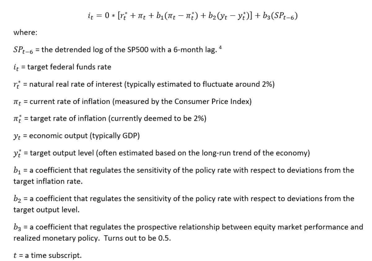
What this equation says is that if you want to know what the Fed will do, rather than what they should do, you need look no further than the stock market. If the stock market has moved decisively below trend over an approximate 6-month period, the Fed is going to cut rates or at least pause any hikes. If the stock market moves above trend, then there’s a good chance they’ll hike or at least stop lowering rates. Everything necessary to operationalize this model, that is to say S&P 500 data, is readily available on an instantaneous basis. Finally, it’s efficacy as a predictive tool is remarkable.
In an associated appendix we present a brief econometric study that examines the, I dare say, “factual’ relationship between equity market performance and Federal Reserve decision making over the last approximately 25 years.
The notable result is that there is a highly statistically significant, lagged correlation between equity market performance and Fed decision making. The 6-month lagged correlation between movements in the stock market (either above or below trend) and changes in Fed Policy is about 0.5 with a so-called ‘p-value’ (a measure of statistical significance) that is vanishingly close to zero, i.e., it is statistically undeniable. Simply put, If the stock market does something untoward, either up or down, then, in about a 6-month timeframe, the folks at the Fed will react by changing course with respect to monetary policy. Playing the role of amateur psychiatrist, I suspect that the causality plays out as follows. The 12 members of the Fed’s Open Market Committee, i.e., the collection of selfless public servants tasked with setting Fed policy, having reviewed their personal 401k statements over an approximate 6-month period, discover that their retirement accounts now look more like 201k accounts. They reach their collective pain threshold and react. The signal they received from the stock market is unambiguous, while the stuff in the Taylor Rule, an elegant collection of stale and/or obscure estimated inputs, is mere commentary. In their defense, the stock market is widely regarded as a very competent forward-looking aggregator of information, so perhaps this is not such a bad outcome.
Looking Forward:
My father, General Weisman, had a great definition of an “expert”, it’s a guy from out of town. I will now pose as an expert.
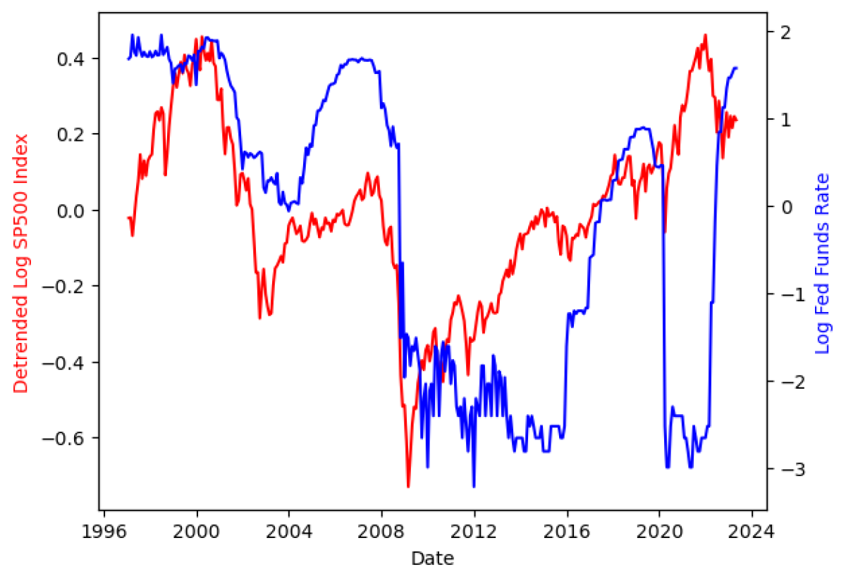
The basic relationship of the stock market to Fed Policy is shown in the “Stocks vs Fed Policy” graphic presented below. By inspection we see that if the log of the stock market moves significantly above or below trend then, in about a 6-month time frame, the Fed will adjust policy. By inspection we also see that the stock market has now moved down a bit (relative to its overall trend). The move has been enough to give the Fed some pause for thought. However, they probably haven’t reached their pain point just yet, but a few more months of scary stock price movement and they’ll cut. Watch the stock market and you’ll know what the future holds for the Fed; in the interim ignore the noise and gratuitous commentary.
Stocks (Detrended Log) vs Fed Policy:
Footnotes:
[1] John B. Taylor, Discretion versus policy rules in practice (1993), Stanford University
[2] "Estimating the natural rate of interest: A review of methods and applications", Thomas Laubach and John C. Williams, Journal of Economic Literature. Link: https://www.aeaweb.org/articles?id=10.1257/jel.20160937
[3] John Maynard Keynes, English economist, and philosopher. He detailed his economic insights in his magnum opus, The General Theory of Employment, Interest and Money, published in 1936.
[4] Detrending data involves removing the effects of trend from a data set to show only the differences in values from the trend. Taking the natural log of a time series provides for a more intuitive interpretation of the coefficients. The coefficients in a logarithmic regression model represent the percentage change in the dependent variable associated with a one-unit change in the independent variable.
About the Author:
Andrew B. Weisman is a Managing Partner and Chief Investment Strategist at Windham Capital Management. Mr. Weisman has more than 30 years of experience as a portfolio manager of alternative investment strategies.
Prior to joining Windham in 2016, Mr. Weisman was the Chief Investment Officer of Janus Capital’s Liquid Alternative Group. Prior to that, he served as Chief Portfolio Manager for the Merrill Lynch Hedge Fund Development and Management Group and Chief Investment Officer of Nikko International.

Mr. Weisman has an AB in Philosophy/Economics from Columbia University, a Masters in International Affairs/International Business from Columbia University’s School of International and Public Affairs, and is Ph.D. ABD from Columbia University’s Graduate School of Business specializing in money and financial markets.
In 2003 he was awarded the Bernstein Fabozzi / Jacobs Levy Award; awarded for outstanding article published in the Journal of Portfolio Management. In 2016 he was awarded the Roger F. Murray Prize (first place) by the Institute for Quantitative Research in Finance for excellence in quantitative research in finance. He is a board member of the International Association for Quantitative Finance, The Institute for Quantitative Research in Finance and previously served for three years as President of the Society of Columbia Graduates.