


By Sorina Zahan, Ph.D., Founder of Aiperion, an R&D, consulting and technology firm that exists to change the way we all think about risk.
Conventional wisdom focuses on volatility as the measure of risk. To this day, allocators are employing volatility in performing essential investment functions such as portfolio construction and investment selection. When stocks and treasuries were all that investors could choose from, the cost of making decisions based on variance might have been small, as the set of choices was small too. Over time though, sophisticated new asset classes and ever-more-complex investment strategies have entered the investment mix. Traditional variance-based methods and metrics have not only become suboptimal, in modern-day investing, they can directly lead to bad decisions.
Why?
At the most fundamental level, using volatility (i.e., the standard deviation of returns) in portfolio decisions has at least three major drawbacks, with significant repercussions on the quality of investment decisions:
- Volatility is a single-period measure—we suggest using path-dependent measures instead
- Volatility is a single-point estimate—we suggest thinking in probability distributions instead
- The relationship between volatility and loss is not linear—we suggest using utility criteria instead
Most allocators are aware of at least the first of these issues. Let’s address all three and propose solutions. Then we will illustrate the framework with a case study.
1. Volatility is a single-period measure … but portfolios are path dependent.
Allocators face the reality that their portfolios are path dependent. Just to give the most common examples, if investors perform rebalancing, if there are portfolio inflows or outflows, or if there are capital calls to fulfill, portfolios become path dependent. Two “identical” return series—i.e., series having the same single-period measures of mean and standard deviation—can produce substantially different paths, depending on their autocorrelation. Note that such identical series will also have identical single-period metrics like Sharpe Ratio, although choosing one series over the over can produce very different results.
Solution
An intuitive, simple and well-known path-dependent measure is drawdown (DD). DD is a peak-to-trough decline in investment value over a specific time horizon (e.g., 10 yrs., 20 yrs.). Investments with positive autocorrelation, such as stocks, tend to have larger drawdowns than investments with negative autocorrelation (e.g., investments exhibiting mean-reverting behavior). Over any time horizon, investments can have multiple drawdowns of various magnitudes. This applies to both historical (realized) DD and to DD modelled in a forward-looking fashion. Maximum drawdown or a lower-rank drawdown becomes a valuable portfolio construction tool, especially when it is modeled for a time horizon consistent with an organization’s portfolio planning horizon. Clearly, this is not the only possible solution, but, because it works so well with investor intuition, it is very easy to use correctly.
2. Volatility is a single-point estimate … but the more illusion of precision a single number gives us, the less knowledge we truly have.
In investing, uncertainty rules. Knowing it is true knowledge. Knowing how wrong a number can be is at least as important as the number itself. In other words, understanding how wrong a model can be is at least as important, if not more, than the model itself. This wisdom applies to any models, independent of how advanced they are, but there is no place where it is more imperative than single-point estimates, the simplest of all models.
Solution
Multiple-point estimates—which can result, for example, from scenario- or sensitivity-type analyses—represent a first step forward. Replacing the single-point estimate with a random variable, which has its own distribution of probability, is an even better option. If we are to use path-dependent risk measures such as DD, this means that we learn to operate with distributions of drawdowns.
It might seem strange to think about volatility, an uncertainty measure itself, as suffering from the single-point estimate problem—i.e., the problem of not knowing how right or wrong that estimate can be. The irony is that, in most financial markets, the uncertainty surrounding this volatility number—the “vol of vol”—is even higher than the uncertainty surrounding the returns. For example, while for the past 20 years the realized standard deviation of monthly S&P 500 returns was 4.25%, the standard deviation of monthly changes in VIX—i.e., the variability of market expectation for the 30-day S&P 500 volatility—was 24.30%. Both are simple, non-annualized numbers.
Therefore, synthesizing the risk (or uncertainty) of an investment in terms of a single number creates a strong assumption dependency in investment analyses. The same holds true not only for measures like downside deviation, VaR, drawdown, etc., either used directly or through the risk-reward type metrics investors commonly use, but unfortunately it also holds true for correlations. Additionally, for most investment types, both volatilities and correlations exhibit strong clustering behavior, i.e., the value today depends on past value(s). This behavior increases the necessity to operate in path-dependent contexts even more.
3. The relationship between volatility and loss is not linear, which means that not all volatility points are equally consequential.
Although volatility is a measure of uncertainty, it is not necessarily a measure of loss or failure.
For instance, it is well understood that by minimizing volatility (for example, in variance-based optimizations), one punishes both gains (upside) and losses (downside). It may be less understood that volatility provides no understanding, nor control, of the negative convexity often found in investments and portfolios, but we will focus on convexity in a separate article.
The fact that volatility is not a measure of failure is less explicitly understood, although, intuitively, it is clear to investors. In our experience working with different organizations, we find they know what actually defines success and failure in their own cases. Further, they understand quite well how acceptable various outcomes are and how acceptability depends on their structure and objectives. In other words, organizations have their own utility functions with respect to risk, and also with respect to reward (1).
The problem starts when one assumes, implicitly or explicitly, that the relationship between volatility and the organization's utility is linear. As you suspect, it is not.
Solution
The logical solution is to use utility criteria in portfolio optimization and investment evaluation. Among other features, utility criteria make practical sense for stakeholders and can be easily fine-tuned by each organization. Intuitive and practical families of such criteria are related to loss (or gain) and failure (or success). In fact, utility can be expressed in many ways and can be efficiently incorporated in the investment process.
For example, the probability of incurring a loss larger than the organization’s tolerance is a basic loss criterion. In this case, the loss metric(s) can be max drawdown severity, and/or duration, and/or steepness, etc. Another example we encounter often across many organization types is the probability that the portfolio value falls below a certain value at any point in time.
Examples of failure criteria include: probability of failing to meet the return target, probability to generate negative real returns, probability to generate returns below a benchmark, probability that the funded ratio falls below a specific threshold at any point in time, etc. All these probabilities should be forward-looking.
Case Study: Asset Allocation Decisions
To put all these points into a practical perspective, we use the case of an institution reviewing its asset allocation. To inform this decision, we performed an AI-based, unconstrained optimization employing utility criteria. Criteria included the probability of suffering, within any 10-year timeframe, a maximum drawdown (maxDD) deeper than -30%, a value which corresponds to the risk tolerance of this organization.
Visualizing the relationship between volatility and the probability of loss P(maxDD<-30%) helps us understand why these decisions should not be made based on volatility. In the two charts below, we separately map the volatility and variance of each optimal portfolio (i.e., each portfolio from the resulting Pareto front) against its probability of loss.
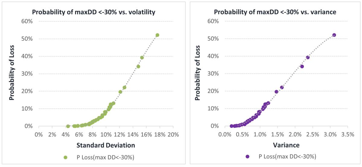
Figure 1. Utility Function: Probability of suffering a maximum drawdown deeper than -30% versus volatility (left) and variance (right) for each optimal portfolio. (Dis)utility increases at a higher pace for higher-risk portfolios.
Clearly the relationship is not linear, i.e., vol points are not equally consequential. Some will be quite benign while others will cause a surge in the portfolio’s chances of facing big losses.
Let’s analyze the decision to change the allocation from a 5.7% return (corresponding to ~9% vol) to one of the two higher-returning allocations:
A. 11% std. deviation, 6.50% mean
B. 13% std. deviation, 7.20% mean
One would think that it is not a big deal to go for B. Who can feel ex-ante the difference between 11% and 13% standard deviation anyway?
The problem is that when vol increases by 2% from ~9% to 11%, P(max DD<-30%) increases from ~5% to 10%. But when vol increases by 2% from ~11% to 13%, P(max DD <-30%) increases from ~10% to 25%. In both cases, the mean return (not shown) increased by ~70-80bp. On the surface, all seems fairly benign. So, what happens?
Essentially, adverse, nonlinear sensitivity to risk (“negative convexity”) kicks in. The extra return, although coming with the same 2% extra vol “cost”, also comes with strongly increasing negative convexity. When bonds and stocks were all we could invest in, the cost of ignoring convexity might have been small. There was not that much hidden behind averages. However, as new assets and strategies (e.g., PE, direct lending, absolute return, factor-based) enter the allocation mix, old methods can lead to increasingly dangerous decisions.
Unwiring Old Wiring
Lastly, a cautionary tale. Let’s think a bit more about the marginal disutility created by moving up the volatility curve above. It is clear that, as we move towards higher “risk”, our chances of loss increase faster and faster.
Now think about the traditional “return over risk” metrics—e.g., ratios such as Sharpe, Sortino, etc. Leaving aside the portfolio vulnerability they can induce by virtue of being single-period, single-point estimates (a limitation which, by the way, is unfortunately often exploited by strategies claiming to be “uncorrelated”), it is worth emphasizing that these types of metrics effectively imply a utility function that is the opposite of what the organization actually cares about—i.e., the higher the “risk”, the smaller the change in these metrics, all else equal (a simple visual contrast between the function 1/x and the disutility function above might help the intuition – see Figure 2).
There are many ways in which this behavior affects our decisions, both pre and post investing. For example, if a return is achieved with higher volatility than expected, the reduction in the reward/risk metric (i.e., the measured disutility) is ~8 times smaller in the 15% risk range than in the 5% risk range. Putting it differently, in order to be indifferent between two options—i.e., measure the same ratio—we require much less compensation if these options are high risk. Therefore, we are induced to make investment decisions against our interest.
Utility incompatibility is costly and should be carefully checked every time a metric of the type reward/risk is considered, no matter how sophisticated it is.
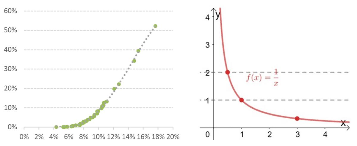
Figure 2. A simple visual contrast between the practical (dis)utility produced for the organization by moving up on the risk spectrum (left) and a (dis)utility function of type 1/x (right).
***
These days, adopting new methods in portfolio construction is not a luxury, it is an imperative. More measurement, more data, more numbers, more charts, and more costs will not make much difference. What is needed is a different way of thinking. As Einstein noted, we cannot solve our problems with the same thinking we used when we created them.
The good news is that, at least based on our experience in working with allocators, it is not difficult to employ the framework we outlined above. Perhaps ironically, because it relies on practical and intuitive solutions to each of volatility’s problems, such framework can actually be better understood and more correctly used than the traditional one.
Reach out to Aiperion at contact@aiperion.ai with comments or for a portfolio review.
Footnotes:
1. For example, in David C. Villa, Sorina Zahan and Brian Heimsoth, 2013: “Analytical Framework for Promoting Pension Plan Structural Robustness and Informed Governance”, we modeled the structural risk sensitivity functions inherent in the main pension structures (DC and DB), as well as in a hybrid plan such as the Wisconsin Retirement System
About the Author:
Dr. Sorina Zahan is the Founder and CEO of Aiperion LLC (www.aiperion.ai), a scientific research, consulting and technology firm that exists to change the way we think about risk because risk measurement is not risk management. Sorina has three decades of scientific research experience in finance, artificial intelligence, and mathematics, and over 15 years of portfolio management experience as CIO.

Previously, she was a Professor at Technical University of Cluj-Napoca, Romania. Her work is focused on creating new practices in portfolio construction, optimizing portfolios directly in the integrated asset-liability space, and expanding the role of AI in institutional investing. Sorina obtained a Ph.D. degree in artificial intelligence in 1997 and holds an MBA from the University of Chicago.