


By David Eichhorn, CFA, CEO and Head of Investment Strategies, NISA Investment Advisors, LLC.
In this paper, we offer a framework to evaluate risk parity manager performance. We begin by exploring the inadequacies of traditional risk parity benchmarking. From there, we look at two alternative benchmarking methodologies based on extracting information directly from manager return data. In one approach, a fixed-weight benchmark is constructed for each manager based on their statistically estimated exposures. In the other, we utilize a rolling evaluation period to provide a dynamic benchmark that adjusts exposures through time with the objective of mirroring the manager’s changes over time. With both approaches, there is no solid evidence of alpha for the cohort of managers. In fact, the average manager underperforms the empirically estimated benchmarks, even after adjusting for the impact of manager fees. Accordingly, we find that passive implementations of risk parity outperform a composite of 17 risk parity managers. We conclude by suggesting that this passive implementation is both a method for identifying a more relevant benchmark for risk parity managers and an accessible investment solution that could be included as part of a risk parity investment strategy.
BACKGROUND
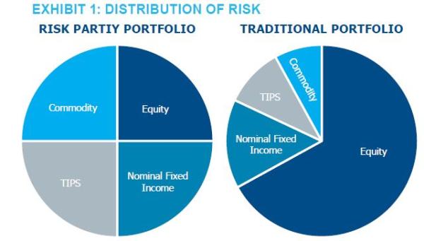
Risk parity, as a strategy, allocates to assets according to their underlying risk characteristics with the goal of generating relatively consistent, high risk-adjusted performance through time. Typically, risk parity managers incorporate nominal fixed income, equities, commodities and inflation-protected bonds (TIPS) into their portfolios in an effort to be more risk-balanced vs. a traditional portfolio, as illustrated in Exhibit 1.
By spreading a portfolio’s risk budget evenly across these asset classes using volatility as a guide, risk parity advocates argue it is possible to generate a higher Sharpe ratio than that of other diversified portfolio constructs, including the archetypal 60/40.
A key component of risk parity’s recipe for success is recognition that utilizing leverage allows an investor to choose the highest Sharpe ratio portfolio (i.e., the mean-variance tangency portfolio) and scale it up to their risk tolerance. In essence, risk parity exploits the key tenets of modern portfolio theory by leveraging the tangency portfolio.1 What makes the risk parity construction unique is that by assuming investments in the portfolio have the same or similar Sharpe ratios, the “optimal” portfolio is an equal risk allocation.2
Regardless of an investors’ view about whether all assets have similar Sharpe ratios, it should be acknowledged that by reintroducing leverage as a tool and normalizing its use, the risk parity construct has been an extremely valuable contribution to the asset allocation paradigm in the 21st century.
Yet, despite commonly held overarching philosophies and underlying asset classes, dispersion in performance across risk parity managers has been substantial. This paper suggests an approach to benchmarking risk parity managers and uses this methodology to analyze whether risk parity managers consistently and systematically generate alpha, i.e., positive returns after adjusting for passive exposures to readily attainable markets, or whether most of their returns are, in fact, simply beta. Spoiler alert — it seems to be the latter.
BENCHMARKING RISK PARITY MANAGERS
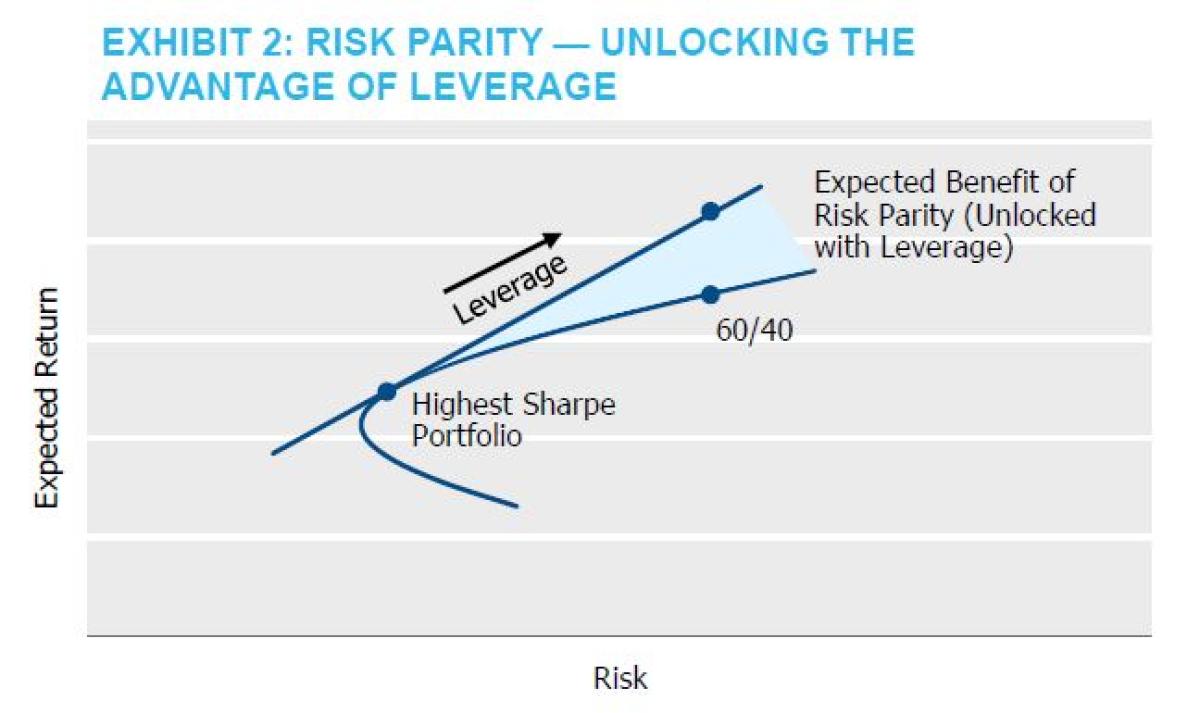
By construction, risk parity is difficult to benchmark.3 As shown below in Exhibit 2, risk parity as a strategy is designed to unlock the shaded region above the classic “efficient frontier.” Asset owners should expect risk parity managers to generate a higher return than points along the frontier (e.g., the 60/40 portfolio), through both a combination of leverage and a different asset blend. Evaluating a risk parity manager’s skill using a 60/40 portfolio of equities and fixed income as a benchmark would be inappropriate as it would be easy to beat over time – both in terms of absolute and risk-adjusted return.
Nonetheless, it is often used in practice due to the lack of readily available alternatives and disagreement over what is a more appropriate benchmark.
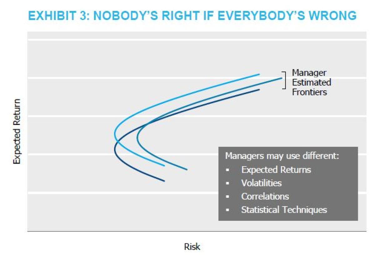
Risk parity is a dynamic asset allocation strategy, shifting as relative risks of assets shift. Measuring whether a manager has designed the dynamic asset allocation strategy effectively is, well, really difficult. The reality is, ex-ante, no one knows the “optimal” tangency portfolio. And every manager has different assumptions about expected returns, volatility, and correlations. Further, managers utilize different statistical methods for deriving these key ingredients that lead to the base portfolio (e.g., highest Sharpe ratio portfolio) to leverage. Additionally, managers may also deviate from each other in regard to enhancement techniques beyond selecting the appropriate base portfolio. This could include tactical asset allocation views, introducing additional asset classes, or other enhancement strategies. That is, each manager creates their own frontier, as stylized below in Exhibit 3, and as lyricized by Buffalo Springfield in 1967, “...nobody’s right if everybody’s wrong.”
At this point, we could take different paths with benchmarking objectives. We could attempt to identify a benchmark based on realized asset class returns that would be useful in evaluating whether one manager made better assumptions than another manager. Aside from being wrought with issues of misinterpretations, this approach effectively demands perfect foresight from the manager universe. That seems unfair...says the investment manager.
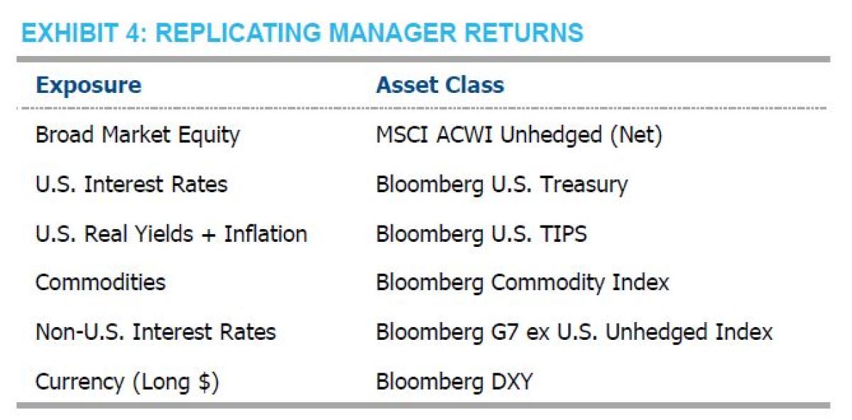
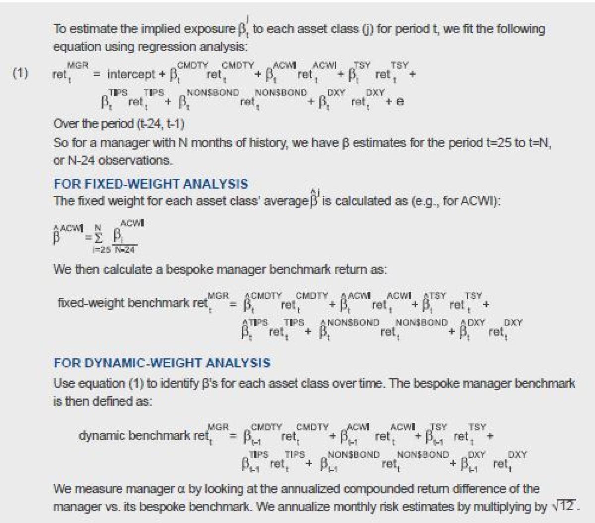
Instead, to identify the implicit levered tangency portfolio of each manager, we suggest an empirical, returns-based analysis. Our approach begins with statistically estimating the holdings of each manager’s levered portfolio. These estimated betas permit us to then measure their incremental value-add. Importantly, we fit each manager to a small, intuitive set of asset class proxies to avoid over-fitting and permit an estimate of their value-add choices (alpha) versus implicit exposures to traditional markets (beta).
INTRODUCING A RETURNS-BASED METHODOLOGY (BESPOKE MANAGER BENCHMARKS)
Throughout this paper, we have used data from HFR Indices (HFR). The data set currently contains a total of 42 managers across 10, 12 and 15-vol strategies thatcomprise the various HFR Risk Parity Indices. The return series are reported net of manager fees. Each manager’s return series varies in length based on the strategy start date, with the first available data beginning in February 2003 and an ending date of December 2021. This provides an ample amount of returns-based data to use in our analysis.5
We took both a fixed and dynamic approach to replicating manager returns using the six main asset classes shown in Exhibit 4.6 A detailed description of the methodology can be found in Appendix A.
FIXED-WEIGHT RETURN ANALYSIS
For the fixed-weight approach, we use the average of our monthly estimated asset class exposures for each manager to calculate the monthly benchmark return for said manager.
By design, this method does not vary exposures over time, but instead represents the manager’s average, “fixed” asset class exposures over the period, as defined by our fitting methodology.
Initially, we performed the fixed-weight return analysis only on current managers with at least five years of continual history. For managers that offer multiple volatility targets (e.g., 10 and 12), we used the lowest volatility strategy to ensure managers with multiple volatility products did not have an out-sized influence on our summary results. To neutralize the impact different amounts of leverage can have, all regressions are performed using excess return time series. This is accomplished by either subtracting the one-month London Interbank Offered Rate (LIBOR) or using an excess return market benchmark. The difference between the manager’s return and the beta-weighted asset class returns can be interpreted as the alpha of the
manager. As you can see in Exhibit 5, the approach does a good job of fitting manager returns, with an average R-squared of nearly 80%. Given the many decision levers at a risk parity manager’s disposal, this was an encouraging indication that it may be possible to benchmark individual managers and, perhaps, even the risk parity community at large.
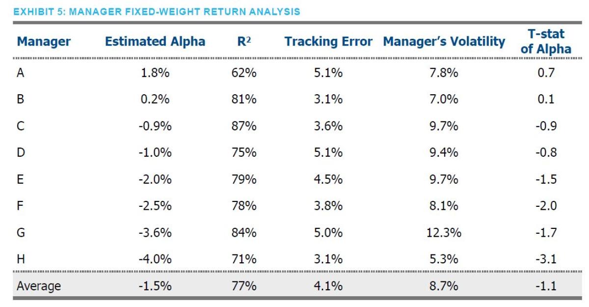
But our key interest is the Estimated Alpha column – suggesting the managers underperformed their fixed weight replicating portfolio by 1.5% on average. Importantly, manager fees, at on average 68bps, only explain a portion of this underperformance.
Looking more closely at the alpha column, two managers (A and B) exhibited positive excess returns compared to the replicating portfolio, while the remainder did not. Importantly, no manager demonstrated a statistically significant alpha, with the highest t-stat being 0.7.
One additional observation is that realized volatilities of manager strategies were broadly below target (Manager A is the only 15% volatility target strategy, while the rest are 10%), an attribute that may not be desirable from the standpoint of an investor. Importantly, our approach does not penalize a manager for underutilization of the risk budget as our tracking portfolio will seek to exhibit similar volatility, all else equal.
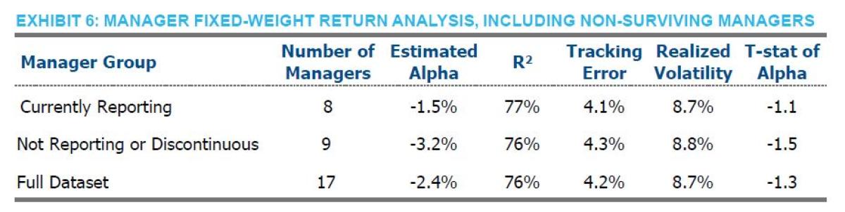
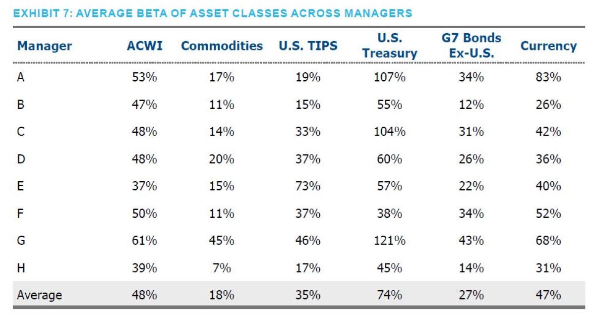
Any statistical analysis would be incomplete, in our opinion, if it didn’t contemplate potential survivorship bias. In order to account for the possibility that the results would look differently if we included managers that either ceased to exist or did not publish during sub-periods, we reran our analysis, including managers that left the index for whatever reason. Exhibit 6 shows that, unsurprisingly, those managers performed worse than surviving managers. As one last sanity check, Exhibit 7 reports the average beta of each of the asset classes across all of the managers included in Exhibit 5. Two observations are immediately evident. First, the weights appear to be very reasonable based on typical descriptions of risk parity implementations – giving us further confidence in the methodology. Second, had an investor held these weights on average over the horizon, they would have out performed the risk parity universe by 1.5%, before any fees and transaction costs associated with this static implementation.
This analysis is, by design, in-sample and provides estimates of alpha in the classic academic sense. That is, have managers demonstrated a skill-based return above and beyond the average market exposures accepted by the portfolio? Of course, given the in-sample nature of this analysis, the outperformance of this approach could not have been realized by an investor historically.7 For that, we need a more dynamic, out-of-sample approach.
MAKING THE RETURNS-BASED ANALYSIS DYNAMIC
In reality, risk parity managers are unlikely to keep fixed weightings to assets over time. So, what if we tried to similarly capture such dynamism in our analysis? Using the prior 24 months to estimate market betas for the subsequent month provides an out-of-sample analysis that dynamically adjusts the exposure weights in an attempt to more closely track managers’ performance.8 Against this dynamic-weight returns analysis, four managers had a positive intercept. In fact, the managers, on average, performed relatively better than they did against the fixed-weight analysis: -0.3% vs. -1.5% (see Exhibit 8). Despite performing better, none of the managers were able to deliver statistically significant alpha.9 Once again, the analysis explains a large proportion of the variation of the managers — nearly 75% on average.
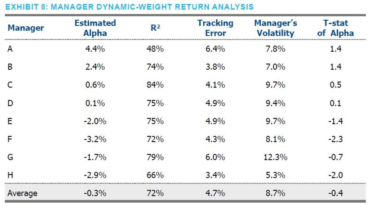
The fact that the managers, on balance, performed less poorly is encouraging on one hand. But, there is a subtle implication when we compare the results of the fixed-weight and dynamic approach for each manager. Irrespective of which returns-based analysis we choose, the manager’s total return is, of course, the same. What changes is the return of our estimated benchmark portfolio. So if a manager’s excess return improves when we perform the dynamic analysis instead of the static version, that is tantamount to saying their dynamic adjustments (as estimated) lowered the portfolio’s overall return. This is another less-than-encouraging sign about the value of the decision-making by risk parity managers. See Appendix C for some additional thoughts on interpreting results from return-based benchmarking.
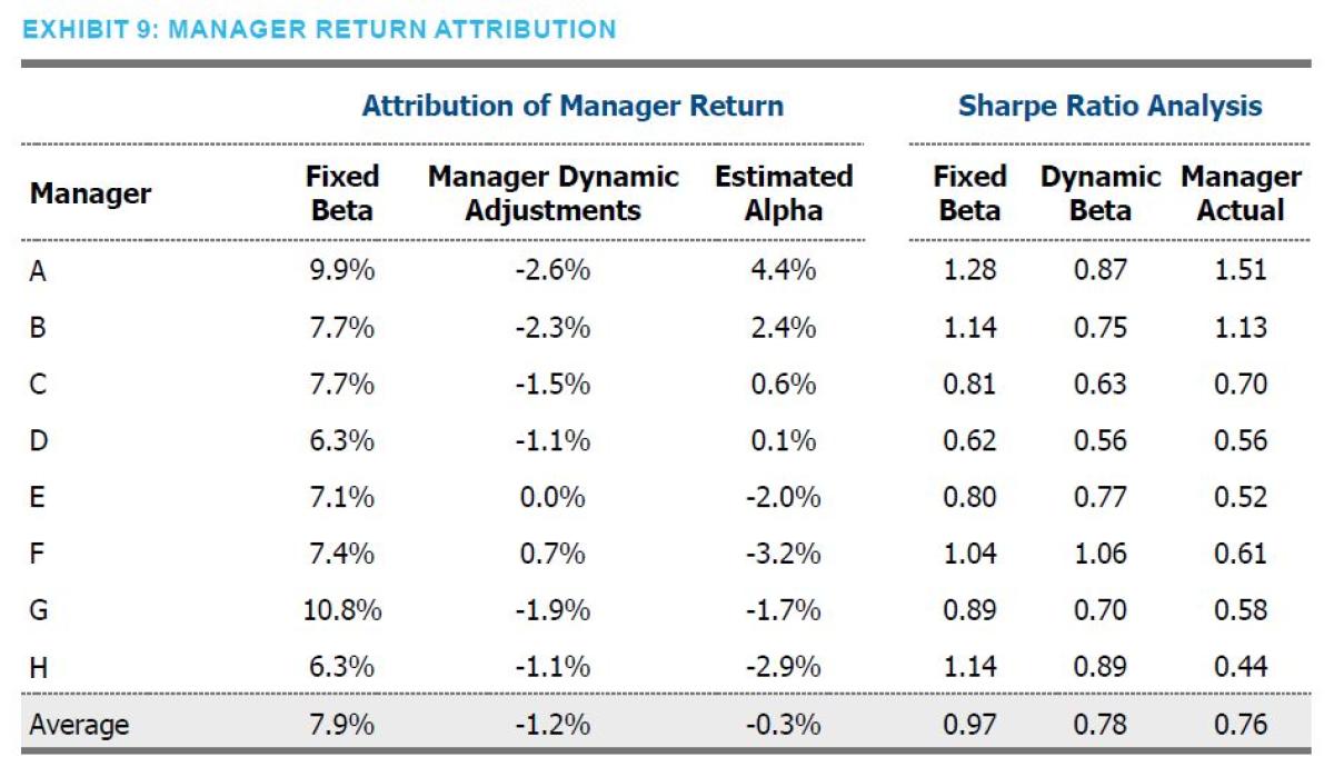
SUMMING UP MANAGER COMPONENT RETURNS: ARE RISK PARITY MANAGERS TRYING TOO HARD?
While the two approaches provide useful insight on their own, combining the two approaches permits an intuitive scoring and attribution of the manager’s performance. In particular, we can decompose the manager's total return into: 1. Manager baseline (fixed) beta return; 2. Manager dynamic adjustment return; and 3. Manager alpha.
Exhibit 9 shows this attribution by manager. The results are quite stark. Using this methodology, the average impact of the managers’ dynamic adjustments is -1.2%. Further, unexplained returns (i.e., alpha) equaled -0.3%.
While there may be a variety of reasons for the dynamic beta adjustments, two common reasons are an effort to keep risks balanced across asset classes and to remain close to the stated volatility target, say 10%. These both may be desirable goals and have a ring of risk management to them. For example, an investor may well prefer their volatility profile to remain constant even when market volatility is rising. Though the analysis above is far from a comprehensive analysis of the root cause of this degradation of return (and such analysis would be a fitting extension of this work), our results at least hint that such volatility targeting may be adjusting exposures at inopportune times vs. expected risk premia. A standard argument for volatility targeting would be that the approach helps clip left-hand tails of distributions. Perhaps. But the Sharpe ratios above suggest otherwise. The managers’ dynamic adjustments reduced the average realized Sharpe ratio (vs. the fixed weights) by approximately 0.2. This reduction in risk-adjusted return was observed in all managers but one, and that manager’s Sharpe went up by a meager 0.02.
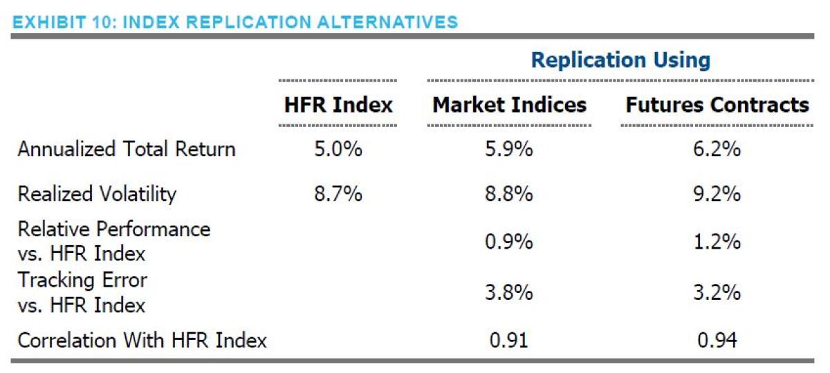
REPLICATING (AND OUTPERFORMING) THE RISK PARITY UNIVERSE
With the dynamic benchmarks in hand, we can easily construct a benchmark that reflects an average of all the managers in
the risk parity universe. Exhibit 10 shows that, indeed, a portfolio can be constructed that closely tracks (i.e., tracking error of 3.8%) and meaningfully outperforms (i.e., excess return of 90bps) the HFR Risk Parity Index™. Furthermore, using directly investable futures contracts instead of published market indices further improves the results – larger outperformance
and lower tracking error. This approach is likely more consistent with what most risk parity managers do in practice. This formulation, being strictly out-of-sample, could indeed have been deployed as a passive alternative to the risk parity managers.10
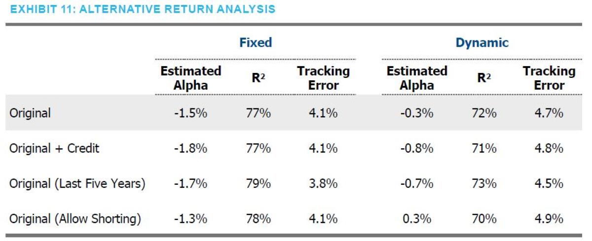
ALTERNATIVE SPECIFICATIONS
Regardless of which approach is used, it is important to confirm that the results hold up to alternative model specifications. When considering other ways to look at the data and explore robustness, we tested the inclusion of credit, different time horizons and allowing for short positions. Exhibit 11 reports the results of each variation in the analysis.
Overall, the results are very comparable to our original analysis. In our opinion, the result of the analysis that permits shorting
should be viewed cautiously, as frequent, outright shorting seems to run counter to the risk parity premise.
In an effort to show as realistic investment results as possible, we replaced the indices shown in Exhibit 4 with directly investable futures contracts. After all, in practice, most managers use futures in their strategies as they are an efficient way to achieve leverage. As implementation costs for futures are more readily identifiable, we also included an analysis that accounts for the transaction costs associated with maintaining futures positions. Results are shown in both Exhibit 10 and 12.
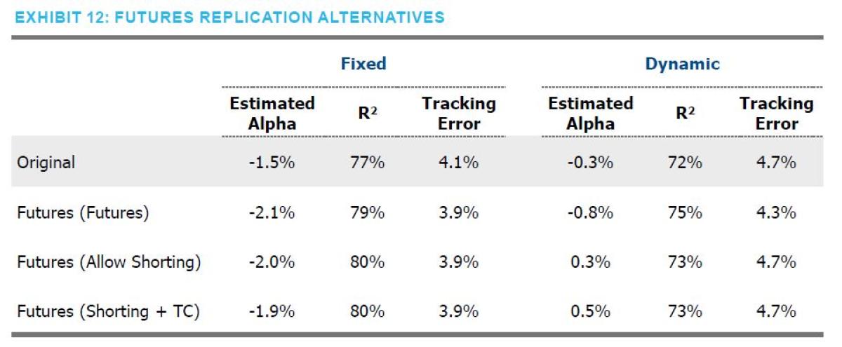
Once again, we believe these results are largely consistent with our baseline analysis, and offers a potentially interesting and easy method of implementing a “passive” risk parity exposure.
THIS APPROACH IN PRACTICE
While we believe our baseline specification is quite suitable in most circumstances, asset owners should modify the approach based on what they understand to be the manager’s style. Modifications might consider the inclusion of additional asset classes (e.g., Gold, energy-focused commodities, EM debt, etc.) or modify the method of analysis (e.g., three-year look-backs instead of 24 months, include volatility forecast as part of the dynamic adjustment process, etc.). That said, we would caution
against the indiscriminate use of additional variables or different approaches. To this day, the admonition of my statistics teacher rings in my head – “with enough variables, I can fit an elephant.” While there is no monolithic definition of risk parity, fundamental aspects of the strategy are likely shared across most managers. A point corroborated by our consistent, high R-squared results. This well-defined arena of risk parity aids the attractiveness of our approach. By contrast, a similar approach for multi-strategy hedge funds would be far more challenging – but fun.
CONCLUSION
Risk parity, as a strategy, has helped many investors achieve higher risk-adjusted returns – in no small part because of the adoption of leverage. But it is important not to confuse this outcome with manager skill/alpha. Our results indicate that investors would have done as well or better by holding the quintessential risk parity asset classes in proportions similar to that of the average risk parity manager’s holdings. Because these weights can be readily ascertained from manager time series either statically or dynamically, we believe that a passive approach exists that investors can utilize to seek better risk-adjusted
performance and undoubtedly lower manager fees.
Footnotes:
All source data for Exhibits 2 - 12 are from HFR Indices and Bloomberg. All data presented in the exhibits are calculated by NISA Investment Advisors, LLC.
1 As a refresher, the tangency portfolio is the portfolio that connects the efficient frontier to the capital market line. This is the portfolio that has the highest return per unit of risk.
2 This is an oversimplification. Asset classes would need to have zero correlation to one another and equal Sharpe ratios for equal risk weighting to be optimal. Whether or not managers actually make these assumptions is irrelevant to the methodology we present here.
3 Please see Appendix B for the role published indices could play in this endeavor.
4 Another challenge is that if a manager uses different asset classes there is the possibility of poor comparisons, and subsequent misinterpretations of “skill” are likely. Please see the appendix for examples of potential misjudgments with respect to manager performance.
5. The raw data set includes 42 managers that were filtered for data quality. We require at least 36 months of return data for each manager. This exposes our analysis to slight survivorship bias. Only 17 managers meet this criterion and only eight of those 17 continue to report returns currently. The impact of this bias is apparent when we compare results of the eight surviving managers to the nine discontinued managers. See Exhibit 6.
6 This set could also be considered five asset classes plus a currency hedge.
7 Though, now that we have exposure estimates for managers (often with long histories), it stands to reason that using these weights going forward could be a reasonable proxy for a manager or the risk parity universe at-large.
8 See Appendix A for more detail.
9 It is perhaps worth noting that Manager A has an outsized impact on the results. Their large relative outperformance and low R-squared suggests they are doing something different, and seemingly better, than other managers. With this outlier in mind, the reader might like to know the median underperformance is -0.8%. Alternatively, removing this manager outright results in an average underperformance of -1.0%.
10 Just because a strategy is out-of-sample does not ensure it could have reasonably been utilized as an alternative to live managers. Finance history is littered with examples of back-test bias in the construction of such analyses that torture data until it inevitably confesses a “strategy.” It is, for this reason, we made what should be evident as extraordinarily limited and simple assumptions for our dynamic benchmark – two-year look-back, common risk parity asset classes, etc. – to limit the likelihood of this bias occurring in our analysis. We believe the reported results here could be improved with refinements, but great caution should be used to avoid the trap of back-test bias.
APPENDIX A
APPENDIX B: A Note on Published Risk Parity Indices
It should be acknowledged that indices have been created to provide an answer on how to benchmark risk parity managers. Both S&P and Wilshire have created investable risk parity specifications at different volatility targets. Following good benchmarking principles, these indices provide investors with transparent and replicable versions of risk parity. However, these indices raise a natural philosophical question – are they an appropriate benchmark to evaluate a given manager or are they simply an alternative specification of a risk parity strategy? We can see arguments for either and, in our opinion, the answer to this question may largely be a matter of taste.
But given the large number of levers at the disposal of a risk parity manager, using one specification of risk parity may be problematic – particularly if the goal is to measure manager alpha over identifiable market betas. Our approach is to provide bespoke manager benchmarks for each risk parity manager. This provides a higher degree of accountability and understanding with respect to the manager. This approach could be used solely for manager evaluation or potentially adopted as the risk parity policy allocation.
APPENDIX C: A Tale of Two Managers
Exhibit 13 illustrates a perfect hindsight approach to returns-based analysis in an attempt to provide insights into a manager’s value-add. It seems clear in this example that Manager B performed better than Manager A.11But did either provide any alpha? We can determine, ex-post, the asset allocation they chose to lever and uncover whether they chose a suboptimal portfolio but added true excess return (true alpha), chose an optimal portfolio to lever but somehow destroyed value through negative excess returns, or underperformed altogether. In a stylized example in Exhibit 14, the benchmarking analysis we propose in this paper could reveal that Manager A chose a portfolio mix to lever that produced a suboptimal shape ratio (empirically estimated leverage line has a smaller slope than ex-post optimal leverage line). But relative to this strategic choice, Manager A provided meaningful excess return vis-à-vis their estimated leverage line, which with further scrutiny, could be deemed true alpha. Manager B however, identified a portfolio mix with a higher Sharpe ratio than the ex-post optimal leverage portfolio. How? Perhaps they included an additional asset class. Their weighting to this additional asset classes did in fact unlock a higher Sharpe ratio portfolio, but other tactical asset allocation or enhancement decisions were made that produced negative excess returns vs. this levered beta portfolio. Manager A and B provide a useful construct and cautionary note on how to interpret the results of a returns-based benchmarking process. Manager A outperformed a poorly constructed base portfolio, while Manager B underperformed a well-constructed base portfolio. How an asset owner evaluates and holds accountable each manager should depend upon what they were expecting from the manager ex-ante.
Managers may outperform because they include assets outside of the assumed benchmark set or employ market timing or other strategies that deliver alpha, and managers may under perform because they incur transaction costs, charge management fees, and/or make poor enhancement decisions. At a minimum, this returns-based framework can help an asset owner understand the decisions that their manager makes and even provide a baseline against which to measure manager performance.
I would like to thank my colleagues, Dan Scholz, Rick Ratkowski and Jeri Glicksman for their work and comments that made this paper possible, and HFR Indices for supplying the data.
About the Author:
David Eichhorn, CFA, the CEO and Head of Investment Strategies, NISA Investment Advisors, LLC.

DISCLAIMER
By accepting this material, you acknowledge, understand and accept the following:
This material has been prepared by NISA Investment Advisors, LLC (“NISA”). This material is subject to change without notice. This document is for information and illustrative purposes only. It is not, and should not be regarded as “investment advice” or as a “recommendation” regarding a course of action, including without limitation as those terms are used in any applicable law or regulation. This information is provided with the understanding that with
respect to the material provided herein (i) NISA is not acting in a fiduciary or advisory capacity under any contract with you, or any applicable law or regulation, (ii) that you will make your own independent decision with respect to any course of action in connection herewith, as to whether such course of action is appropriate or proper based on your own judgment and your specific circumstances and objectives, (iii) that you are capable of understanding and assessing the merits of a course of action and evaluating investment risks independently, and (iv) to the extent you are acting with respect to an ERISA plan, you are deemed to represent to NISA that you qualify and shall be treated as an independent fiduciary for purposes of applicable regulation. NISA does not purport to and does not,
in any fashion, provide tax, accounting, actuarial, recordkeeping, legal, broker/dealer or any related services. You should consult your advisors with respect to these areas and the material presented herein. You may not rely on the material contained herein. NISA shall not have any liability for any damages of any kind whatsoever relating to
this material. No part of this document may be reproduced in any manner, in whole or in part, without the written
permission of NISA except for your internal use. This material is being provided to you at no cost and any fees paid
by you to NISA are solely for the provision of investment management services pursuant to a written agreement.
All of the foregoing statements apply regardless of (i) whether you now currently or may in the future become a
client of NISA and (ii) the terms contained in any applicable investment management agreement or similar contract
between you and NISA.