
By Roberto Croce, Head of Risk Parity and Alternative Risk Premia, Newton Investment Management North America LLC.
INTRODUCTION
Inflation hedging is of particular interest to investors today, as recent consumer price inflation numbers show inflation rising faster and higher than at any time since the global financial crisis more than a decade ago. In this paper we answer the following questions:
Question 1. Does inflation only matter to investors with liabilities denominated in real dollars?
Answer 1. No. We find that the hedge/no hedge decision does not depend on whether investor liabilities are denominated in real or nominal US dollars. In this paper we will show that high inflation periods are almost as bad on a nominal basis as they are in real terms, particularly when the cash return is zero.
Question 2. Is gold an effective option for investors who want to hedge inflation?
Answer 2. Empirical evidence shows gold may not be a reliable inflation hedge. We believe there are some broad commodity investing approaches that are more likely to deliver good results. The key point of this paper is that investors relying on precious metals to hedge inflation could be disappointed. Our estimates suggest inflation surging to 5% would lead to precious metals performance of roughly cash plus 5% (cash plus 0% on a real basis), whereas well-crafted broad commodity portfolios could earn more like cash plus 15% in such an inflation surge. In addition, broad commodity exposure can be designed so that it still works in disinflationary environments, with expected returns of cash plus 3.5% in a 2% inflation world.
Question 3. How can we build a strategic asset allocation that accommodates multiple inflation scenarios?
Answer 3. One effective method is to shift historical means of asset returns and inflation to reflect forward-looking investment views, then build optimal portfolios based on the new distribution of asset and macro data. We provide a basic example of how to do this in the final section of the paper. One result that stands out is that the low expected return on bonds today makes the opportunity cost of owning inflation-sensitive assets much lower than it has been historically and increases the optimal exposure to these assets across multiple portfolio objectives.
The paper also provides historical perspective on real returns of stocks and bonds during the inflationary episodes of the 20th and early 21st centuries by first identifying periods of high inflation and then examining the performance of stocks and bonds during these periods. Consistent with the typical narrative, both stocks and bonds generate a negative real return during most inflation episodes. But importantly, they also underperform cash in these environments, making inflation hedging an important concept, even to investors with objectives denominated in nominal terms.
With this in mind, we extend the analysis to the performance of gold, broad commodities, and Treasury Inflation-Protected Securities (TIPS) back to the early 20th century. We find that broad commodities performed a bit better than gold on average during inflationary episodes, and gold was only really helpful during the inflation episodes in the 1970s. TIPS were good at hedging their own cash flows against inflationary pressures and outperformed cash on a real basis, but the outperformance was not so material that an investor could use TIPS to hedge their broader portfolio against inflationary shocks.
Next, we take a deeper look at gold performance during inflationary episodes, with an eye toward understanding why it was so strong in the 1970s but has seemed much less related to inflation since then. Statistically, the correlation between gold prices and inflation was strongly positive in the 1970s (+0.36) but has been virtually uncorrelated (-0.03) since 1981 (Bloomberg, accessed 10/1/21). It is important to note that gold’s strong performance came in the decade after the gold standard was abandoned, when the US dollar depreciated tremendously against gold. All developed market currencies that were part of the Bretton Woods system depreciated relative to gold during the adjustment period. We think this is an important detail to keep in mind and we include a detailed discussion of it in part three of this paper. The conditions that made gold work so well in the 1970s are simply not present today.
Commodities that comprise the raw materials put into production processes have had a much more reliable relationship to inflation that has persisted throughout the historical period of study. Statistically, the correlation between broad commodity prices and inflation was strongly positively correlated to inflation before 1980 (+0.35) and has been similarly strongly correlated since 1981 (+0.31) (Bloomberg, accessed 10/1/21). The problem with broad commodities is that they have generated low or even negative returns over the last three-plus decades, a period during which the US has experienced very little inflation.
In the final section of this paper we use standard portfolio construction concepts and some first principles of commodity futures markets to design what we believe to be a structurally superior commodity strategy that has the potential to generate returns in the neighborhood of cash plus 3% in a benign inflation environment, with expected returns that scale at over three-to-one relative to inflation, and an expected nominal return of cash plus 30% if inflation hits 10%. Precious metals, by comparison in the same framework, are expected to generate cash plus 4% in a benign inflation environment, with a nominal return of cash plus 7% if inflation hits 10%. If history is a guide, then precious metals may almost keep up with inflation but will not provide a substantial hedging benefit to a broader portfolio.
Part 1: Historical Market Performance during Inflation Episodes
Why would investors consider an explicit allocation to inflation hedging assets? The conventional wisdom is that traditional stock and bond investments typically do very poorly during inflation episodes, particularly on a real (net of inflation) basis. In this section of the paper, we identify the notable inflationary episodes of the 20th and early 21st centuries, and then look at as much data as possible on the performance of stocks and bonds during these episodes. Our analysis supports the conventional wisdom. We extend the analysis by looking at some typical inflation-hedging assets: TIPS, gold, and broad commodities.
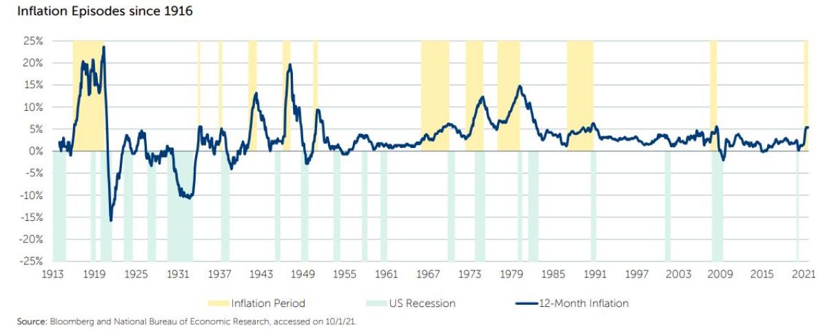
Our historical study starts with a quantitative definition of what defines an inflation episode. We tried several approaches and they all led to qualitatively similar results. Here we will define an episode as any rolling 12-month period in which all the following are true:
- Inflation is over 2%
- Inflation eventually rises to over 5%
- Inflation is at a peak or has not yet peaked
- Inflation has not fallen by more than half of its episode peak
- Cumulative inflation is 5% or more
We believe that this methodology identifies episodes where inflation is rising and is at a material level. The figure below shows rolling 12-month inflation, with yellow bars indicating inflation episodes and green bars representing recessions as defined by the National Bureau of Economic Research. It should be noted that two periods in the 1930s when rolling one-year inflation crossed 5% are not designated as inflation episodes because cumulative inflation over the windows of interest was not greater than 5%.
Next, let’s study the performance of stocks and bonds during these episodes, net of inflation, and compare them with cash to answer the question: do risk assets outperform risk-free investments on a real basis during inflation episodes?
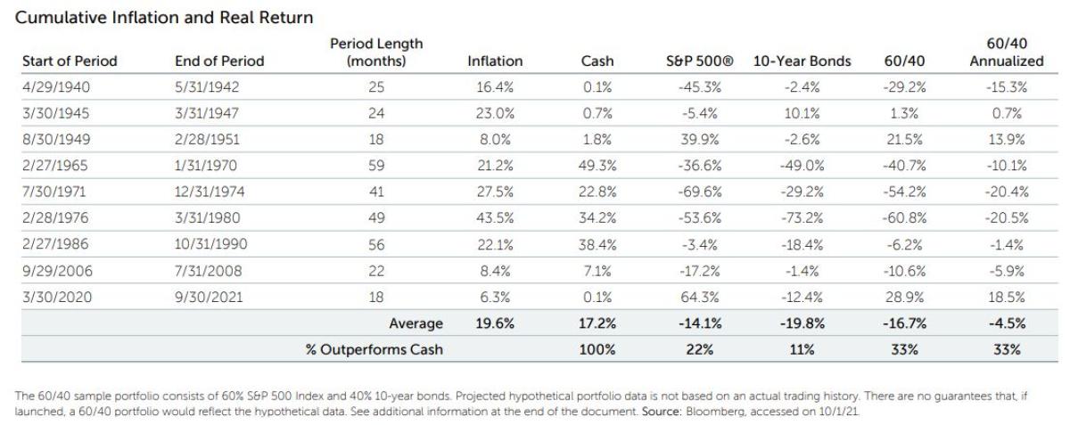
A couple of comments on the dataset itself. Unless otherwise noted, all data in this paper is downloaded from Bloomberg. Inflation data comes from the Bureau of Labor Statistics and begins in 1913. Inflation episodes are identified retrospectively using the method described above, and cumulative inflation during the episodes is subtracted from cumulative excess return on the asset, then cash is added to the asset return. Where S&P 500® or “stocks” data is referenced, it represents the total return index beginning in January 1988. Between 1971 and 1988, total return data is proxied by price return plus 1/12 of trailing 12- month dividend yield. Prior to 1971, S&P 500 total return is proxied by price return plus 3% per year. The stock price data begins in December 1927 and starts appearing during the 1940s inflation episodes.
We derive our bond returns from a time series for ten-year bond yields that begins in January 1962, backfilled with composite data from the Federal Reserve Board for bonds with over ten years left to maturity to January 1925. We assume a new bond is struck each month that earns a monthly coupon of the prior month’s headline yield/12. The value of the prior month’s bond is calculated using this month’s yield as a discount rate. The total return on the prior month’s bond is 1/12 the prior month’s yield-implied coupon (a yield of 5% implies an annual coupon of $50 on a $1,000 face-value bond) plus the new price of last month’s bond divided by 1,000. Our cash return data is US 3-month T-bill rates from January 1954 onward. Prior to 1954, we backfilled with short-term fixed income rates from the Ken French data library back to July 1927.
Consistent with the conventional wisdom, stock prices fell on a real basis in five out of nine inflation episodes (56%) and bonds fell in six out of nine (67%). Relative to cash, both stocks and bonds outperformed in five out of nine episodes (56%), but a combination of 60% stocks and 40% bonds (60/40) outperformed cash only 44% of the time during inflation episodes. The average length of inflation episodes was 34 months, or almost three years. Investment policies that systematically underperform cash under certain conditions— conditions which tend to last three years at a time—are policies that can be improved upon.
In the next section, we will extend the inflation event study to include the assets that most commonly come up during discussion of inflation protection: TIPS, broad commodities, and gold.
Part 2: Inflation Asset Performance during Inflation Episodes
In this section, we assemble the longest possible datasets for inflation-linked bonds and a number of single and aggregate commodity indices to understand their relative performance during inflation episodes. As we will show, TIPS may effectively hedge their own cash flows, but they certainly do not generate enough additional return during inflation episodes to consider them a hedge for a broader portfolio. Gold performed very well during the inflation episodes in the 1970s but had virtually no relationship to inflation after 1980. Broad commodity prices, on the other hand, rose more than one-for-one with inflation in every inflation episode for which we have data. Naïve commodity indices, which differ from raw commodity prices due to the accumulation of roll yield over time, rose more than one-for-one with inflation in four out of five episodes.
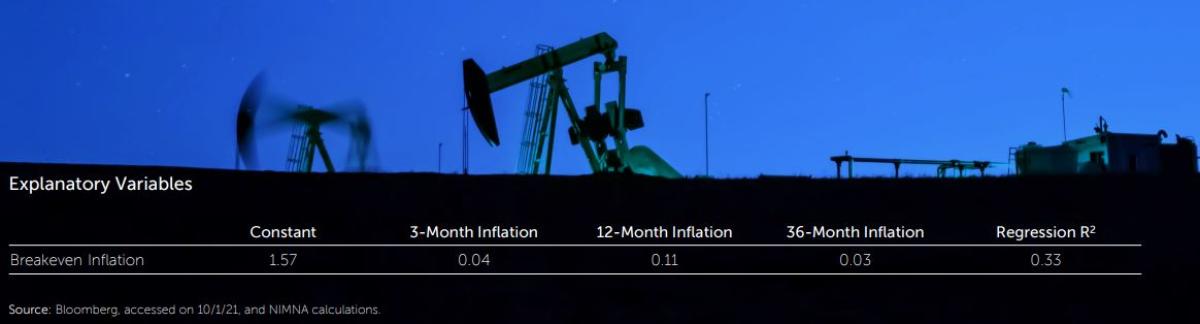
The US Treasury began issuing TIPS in 1997. As such, there is no direct return stream available prior to 1997. But we can still draw some inference about what TIPS might have done historically if we can figure out how their prices systematically relate to nominal bonds given current and historical levels of inflation. In order to answer this question, we regressed breakeven inflation rates, which are the rates of future inflation that would exactly equate the yield of nominal bonds to the yield of TIPS, on lagged three-month, 12-month, and 36-month realized inflation and a constant. The results of the regression are shown in the table below. The results show that, on average, breakeven inflation is positively related to three-month, 12-month, and 36-month historical inflation rates, with changes in inflation over the last year being the largest contributor to expected fluctuations in the breakeven rate.
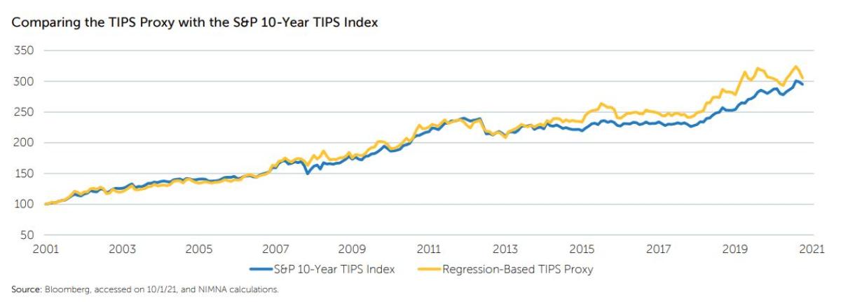
The regression allows us to project expected breakeven inflation rates back in time to 1916 by feeding inflation information through the model. Next, we proxy for real interest rates by subtracting the fitted breakeven rates from historical data for nominal rates in order to arrive at a proxy for historical real rates. These model-based real rates can then be converted into implied price changes for TIPS. To get a sense of the accuracy of this methodology, we compare the returns of the S&P 10-Year TIPS Index with the returns from our methodology; the correlation between the two series is 72% and the cumulative return of both series is plotted below. The fit of proxy TIPS return series is very good and captures the inflation period in 2007-2008 particularly closely.
Alongside TIPS, we consider broad commodities and gold. The table below shows the real (adjusted for inflation) performance of gold prices, an index of commodity futures and stock prices, as well as our proxies for bond and TIPS total returns in every period for which we have good data back to 1916. Referring to the table, real gold returns were the exact opposite of the inflation rate for all the episodes before 1970. This is because of the gold standard, a process by which the federal government fixed the value of the US dollar relative to gold. Only after the abandonment of the gold standard did the price of gold float relative to the US dollar. Subsequently, gold performed very well during the inflation episodes beginning in 1972 and in 1977, returning 321% and 230%, respectively, on a real basis. Consumer prices rose 28% and 44% in these two episodes. In the more minor inflation episode beginning in 1986, gold lost 10% of its value on an inflation-adjusted basis. In the inflation episode that preceded the global financial crisis, gold gained 44% on a real basis. In aggregate, gold generated an average return of 58% during inflation episodes (119% post gold standard), but this respectable performance is dominated by the 1970s inflations. Gold appreciated in three of the five inflation episodes for which we have data, for a hit rate of 44% (80% post gold standard). The worst real performance by gold was -10% during the inflation episode that began in 1986.
The 1970s inflation episodes were among the most meaningful in this sample, and any good inflation hedge needs to perform in that environment. But the 1970s were also unique in that they occurred just after the United States abandoned the gold standard. We discuss the possible implications of this observation in a later section. Outside of the 1970s, the inflation-adjusted performance of gold was very mediocre during inflation episodes.
Commodities, as measured by the Bloomberg Commodity Index (BCOM), appreciated in every inflation episode, even when adjusted for inflation, giving them a 100% hit rate. The average performance of commodity prices was 134% across the inflation episodes, and the worst inflation-adjusted performance was 20.9%.
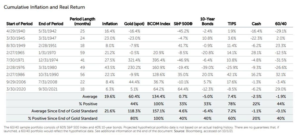
Using the proxy method described above, we are able to evaluate the likely performance of a basket of TIPS during the same episodes for which we have nominal bond returns. It is interesting to notice that TIPS do an admirable job hedging inflation relative to their nominal bond siblings, generating an average real return of 7.4% instead of -5%. But the magnitude of TIPS returns certainly would not have been sufficient to offset the poor performance of stocks and bonds during the inflation episodes shown here. For that, one would have needed commodities, and specifically, broad commodities.
Part 3: Unpacking the Great Gold Performance of the 1970s
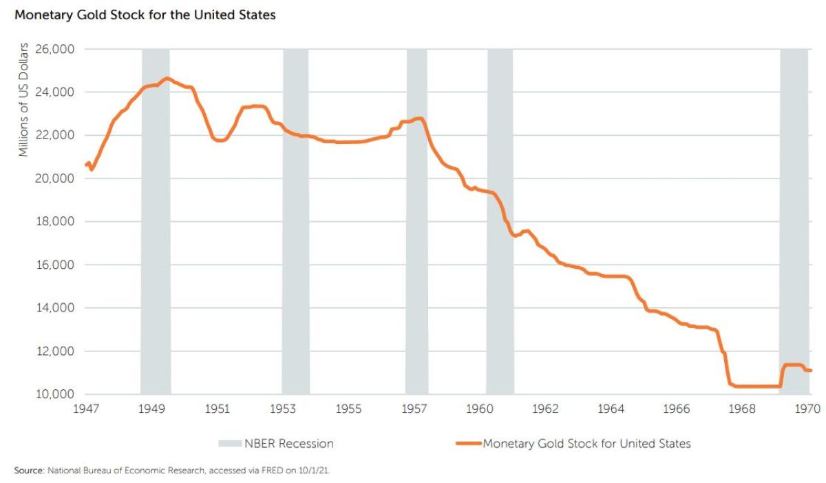
It is important to note that the great inflation of the 1970s was immediately preceded by the final abandonment of the gold standard on August 15, 1971, when Richard Nixon announced that the United States would no longer redeem currency for gold. Prior to this announcement, the US dollar price of gold was fixed, and many other countries pegged their exchange rate in terms of dollars. In fact, the dollar price of gold was being held artificially low by the guarantee of explicit convertibility into US dollars at a fixed rate. The figure below shows that gold on deposit at the Federal Reserve to support convertibility plummeted between 1949 and 1970, and when it became clear that convertibility could not be sustained indefinitely, the peg was abandoned, and the price of gold subsequently rose relative to all major currencies.
Over the following decade, gold prices rallied dramatically relative to the US dollar. In other words, US dollars and the currencies of other Bretton Woods nations lost purchasing power dramatically relative to gold. It is not surprising, then, to learn that the price inflation of goods was high during this period, as the value of fiat currencies fell to adjust for the abandonment of convertibility to gold.
Statistically, we find that gold prices and inflation were correlated at +0.34 between 1967 and 1980. Interestingly, gold had a large negative correlation of -0.51 with the US Dollar Index as well, while the US Dollar Index and inflation were totally uncorrelated.
Studying only the period after 1980, the relationship between gold and inflation disappears totally and the correlation measures -0.07. There is no discernible relationship. But the relationship between gold and the US Dollar Index remains and has a similar magnitude of -0.43 relative to the earlier period. Thirdly, inflation and the value of the US dollar were statistically unrelated. We interpret this fact pattern to mean that, in general, gold is a pure play short the US dollar. In the 1970s, currency depreciation resulting from the abandonment of the gold standard was a significant driver of inflation in the Consumer Price Index. In addition, the US Dollar Index is the price of the US dollar relative to a basket of other developed currencies. Because many developed currencies had also been de facto pegged to gold through their peg to the US dollar, it is not surprising that a portion of the inflation should appear to be totally unrelated to the price of the basket of currencies.
Given the proximity of outstanding gold performance to the end of US dollar convertibility to gold, we think it likely that the price of gold had been held artificially low for an extended period (or the price of US dollars was held artificially high) and that the subsequent abandonment of convertibility drove an adjustment period both in consumer prices and in the price of gold relative to the US dollar. In other words, abandoning the gold standard was in part causative of inflation and of the increase in gold prices. The great increase in gold prices in the 1970s was not some endogenous macroeconomic response to inflation—it was the direct result of the same event that drove a portion of the inflation. In the absence of a gold standard, the adjustments in consumer prices and in gold would probably have taken place over a longer period and in a less disruptive way—the gold standard acted as a dam holding back natural economic forces. But as pressure mounted, the dam eventually broke (the US ran out of gold with which to support convertibility), leading to a much more disruptive adjustment.
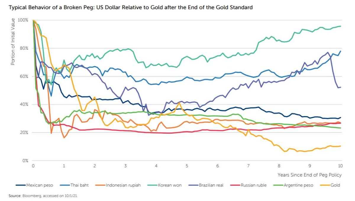
The figure below shows the value of US dollars relative to gold starting at the point when the gold standard was discontinued in August 1971. Alongside this, we show the value of various foreign currencies after their pegs against the US dollar were abandoned. The point is that the pace and magnitude of US dollar devaluation is typical of a broken currency peg. Pegs break because natural economic forces push on them. In the case of the gold standard, it was lack of availability of gold with which to support convertibility. When currency pegs break, it is because of a shortage of the reference currency with which to defend the peg. During initial defense of the peg, the economic forces build such that when the peg eventually breaks, the moves are very substantial. We believe that the end of the gold standard was the primary driver of strong gold performance in the 1970s, and that the inflation hedging benefits of gold in the 1970s were essentially coincidental. Certainly, the conditions for a repeat of this performance are not in place today. So, what can we reasonably expect? We will unpack this in the next section.
Part 4: Designing a Commodity-Based Strategic Inflation Hedge
In the sections above we showed that the real and even the nominal returns of stocks and bonds are negatively affected by inflation, implying that all investors should attempt to hedge inflation if the cost does not outweigh the benefit. The purpose of this section is to explore some common features of commodity futures markets and try to understand the potential opportunity cost associated with an allocation to commodities. Some key empirical features of commodity markets, on average, across current constituents of the Bloomberg Commodity Index, are:
1. Very lowly correlated to one another, with average cross-commodity correlation of 0.22.
2. Relatively low return, and historically have generated an arithmetic, average excess-of-cash return of 2.3% per annum since 1991.
3. High volatility, with single-commodity riskiness averaging 27.5% per annum. High risk and low arithmetic average return together suggest that the average single-commodity geometric return should be materially negative, and it is (at -1.5% per annum).
4. Embed a substantial cost of carry, particularly in near-dated commodity futures.
Feature 1 above indicates that there is likely to be a significant diversification effect from combining commodities in a portfolio. This diversification would reduce the volatility of a diversified commodity portfolio materially, and in fact it does. While the average single-commodity volatility is 27.5%, the volatility of the diversified index of commodities is only 14.5—just a bit over half as risky. This risk reduction alone will help close the gap between arithmetic and geometric return.
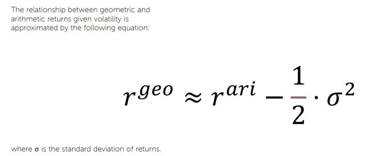
We can use this relationship to help understand why the geometric return of the diversified commodity portfolio is so much better than the average geometric return across markets—its risk is much lower, so the geometric return is higher. So, while the empirical feature 3 (above) implies a large gap between arithmetic and geometric returns for a single commodity, the risk reduction facilitated by empirical feature 1 dampens the risk of a portfolio of commodities and boosts geometric expected return. On average, the risk reduction from diversifying a portfolio of commodities is sufficient to add about 3% to the geometric return relative to a riskier single-commodity portfolio at the same arithmetic return (0.5*(27.5%^2-14.5%^2) = 2.94%). In fact, the optimal commodity portfolio for an investor with no views as to the relative attractiveness of one commodity versus another would allocate equal risk across commodities, in the manner of risk parity. The risk parity portfolio has risk that is about 1% lower than the Bloomberg Commodity Index, resulting in an even smaller gap between geometric return and arithmetic return.
The fourth empirical feature noted above is that commodity markets embed a cost of carry, often called a “convenience yield.” A convenient means for thinking about cost of carry is through the lens of zero-arbitrage conditions, which are the series of physical market-replicating transactions. In efficient markets, the futures market price of a commodity will be very similar to the combined cost of a series of transactions: borrow the capital to buy the physical commodity and all related costs, buy the physical commodity, pay to store the commodity, and then deliver the commodity to the standard delivery point at contract maturity. If there is a material difference between the price of the physical replication and the current futures price, arbitragers will buy the cheap leg and sell the expensive leg to earn a risk-free profit. It is a basic principle of economics that the supply of most things is relatively fixed in the short run, becomes somewhat more flexible in the intermediate term, and is totally elastic in the long run. This is certainly true of the cost of storage.
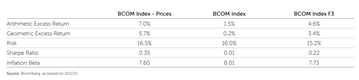
Consider an investor who needs to store a large quantity of corn tomorrow. The cost could be very high because of the immediacy of the need, whereas the cost could be materially lower when arranging storage for corn starting one month from today. In addition, an investor that has to deliver a physical commodity at the end of the current month will incur transportation costs in the near term. These costs typically are reflected in commodity futures as a higher cost of carry in nearer-dated futures. Historically, the impact of this cost of carry, has been about -5.5% per annum since 1991, as shown in the table below. So while commodity prices rose at 7.0% per year on average, investors cannot invest directly in a basket of commodities without incurring costs associated with storing and transporting them. Even if you held the physical commodities and avoided the cost of carry embedded in futures, you still would have had to pay to transport and store the physical commodities. Net of these costs, returns would have been disappointing. In our opinion, this is why most investors have abandoned commodity allocations.
The convenience yield embedded in futures contracts declines as you begin to look at longer-dated contracts, much like the time decay of options decreases as you increase the time to maturity. Simply rolling contracts a quarter further out (BCOM Index F3) improves historical geometric return by 3.2% (from 0.2% to 3.4%). Unlike in equity options, the hedging potential of the deferred contracts is virtually identical to that of the nearer-dated maturities, evidenced by the inflation beta of 7.73 for the deferred index.
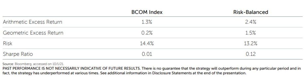
Bringing all of these empirical observations together into a single concrete optimal commodity strategy, we recommend a straightforward implementation of risk parity across all liquid commodity futures markets, implemented one quarter out relative to the front-month contract in markets where there is liquidity at that curve position (risk-balanced deferred). The benefits of maximizing diversification and reducing the cost of carry embedded in the futures portfolio combine to improve historical geometric return by over 3% per year relative to a naïve BCOM futures replication. Implementation of this strategy is simple and inexpensive, and with a historical return of cash plus 3.6% in what can only be called a challenging environment for commodities, we think this is an attractive proposition for inflation-sensitive investors.
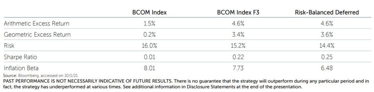
The inflation beta of the more diversified commodity portfolio is a bit lower: 6.48 versus 7.73 relative to the deferred BCOM exposure. This result is driven by a larger allocation to agricultural commodities, which are a smaller portion of the BCOM Index than of the more diversified risk-balanced approach. Even with this in mind, we believe the diversified approach is more attractive. The most obvious reason is that diversification occurs in the risk-balanced portfolio construction by design, and it should remain diversified no matter what the relative allocations of the BCOM Index become in the future. The second reason is that the probability distribution of outcomes for the risk-balanced approach is significantly more defensive—in cases where high inflation doesn’t materialize, the approach is more robust. The table below shows the results of a regression model that relates portfolio returns to inflation and changes in the value of the US dollar. Assuming no change in the value of the US dollar, the model allows us to form expectations about how a portfolio might perform at different rates of inflation based on the historical regression relationship between January 1990 (when the deferred commodity indices become available) and September 2021, and the inflation rate.
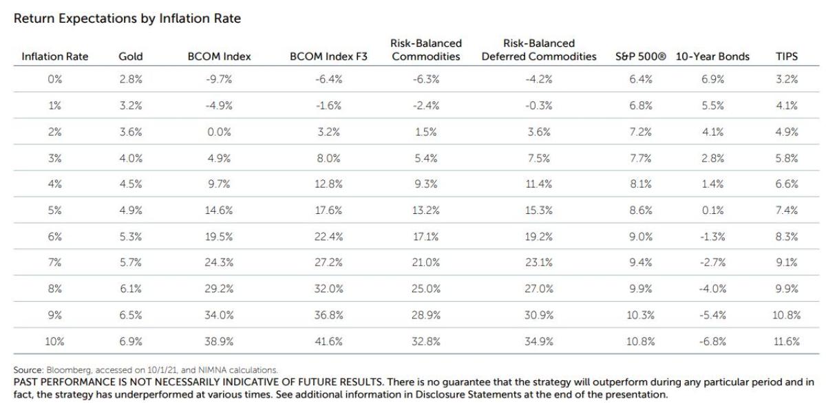
The key observation is that at inflation rates of 2% or less, the risk-balanced approach generates much better returns. We think that this characteristic makes it the more attractive strategic allocation for investors that want to hedge inflation without locking in a negative return if the environment turns out to be more benign.
It is also interesting to notice the conditional expected behavior of the other markets shown in the table. Front-month commodities generate excess return of -4.9% when inflation is 1%, and do not begin generating positive expected return until inflation moves above 2%. No wonder naïve commodity allocations have been so difficult for investors to maintain over the last decade, when realized inflation was less than 2% per year. Gold generates positive excess nominal return across environments, but, if you subtract the inflation rate, the real return falls into negative space at 5% inflation. Gold is not sufficiently inflation sensitive to generate a high positive real return during inflation episodes, and therefore it is likely that it cannot be relied upon as a hedge for the broader portfolio. According to the table above, stocks also are unable to keep pace with inflation, and real return falls below 1% when inflation hits 10%. But they keep up effectively on a nominal basis. Bonds display exactly the kind of relationship to inflation that they are purported to, and even nominal returns turn negative before inflation hits 6%—meaning -6% on a real basis. The table shows an outcome consistent with the result earlier in the paper, suggesting that TIPS hedge their own cash flows effectively against inflation, but that there is not enough return on a real basis to offset losses elsewhere in a portfolio.
Part 5: A Framework for Considering the Optimal Allocation to an Inflation Hedge
The key finding is that intelligently implemented broad commodities make up a substantial portion of the optimal allocation under most objective functions, both using historical data and when applying forward-looking return assumptions. These results are true for both nominal- and real-return investors. Some objective-function/return-assumption combinations allocate substantially to gold, others do not; some favor inflation-linked bonds, others nominal bonds. But substantial allocations to equities and broad commodities are robust in relation to almost any parameterization.
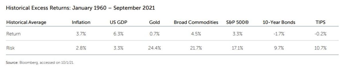
How can this be? Isn’t the conventional wisdom that commodities generate zero return above cash, even though they hedge inflation? The punchline is that an intelligently implemented commodity portfolio has done pretty well. Specifically, since January 1960, the average rolling 12-month real excess return and risk across the asset classes discussed here are as follows:
In order to facilitate a dataset of this length, we’ve had to extend the proxy for intelligent commodities and for equity total returns back in time.2 We are also using a regression-based model to infer a proxy for breakeven inflation and extend the inflation-linked series back in time. We consider three illustrative objective functions:
1. The portfolio with the best outcome at the 10th percentile of realized one-year returns
2. The portfolio with the highest median total return
3. The portfolio with the highest risk-adjusted return.
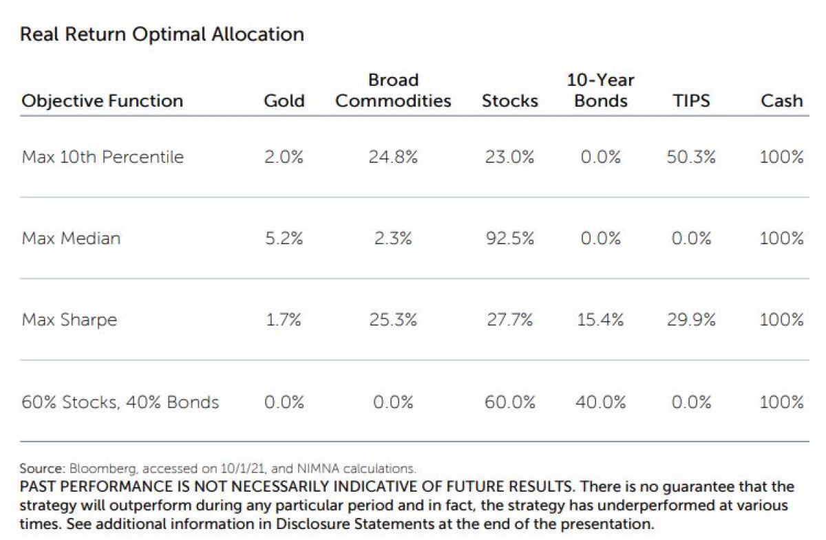
Because we are using time series and solving numerically for portfolios based on the empirical distribution of historical returns, this methodology preserves the conditional correlation properties of the underlying assets in different economic environments and allows us to solve for very different optimal portfolios under real- and nominal-return objectives. There are a number of interesting implications from the optimization results, but the most critical one for our purposes here is that every single optimal portfolio included at least 9.5% commodities, regardless of whether investors sought real or nominal returns. By contrast, gold made up only between 0.0% and 2.1% of the optimal allocations, depending on which objective function and inflation treatment was applied.
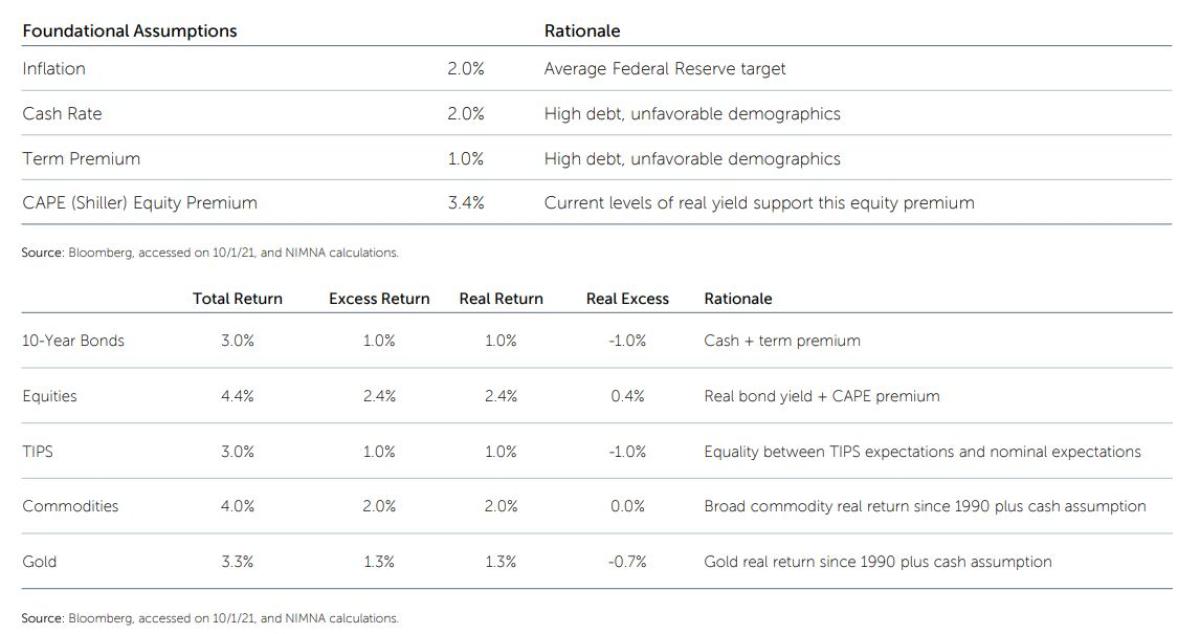
Certainly, this result is driven at least in part by the strong performance of the broad commodity series over this time period. It is important to keep in mind that the price of gold was effectively pegged to the value of the US dollar prior to August 1971, meaning the real return of gold was zero prior to that time and the real excess return was minus one time the return on cash. So perhaps the return on gold is unrealistic over the time period studied. Further, much of the study included periods of much higher inflation than anything seen in the last few decades, so perhaps the return assumption for broad commodities is too high. Stocks and bonds are both quite expensive as of this writing, so maybe those expected returns need to be adjusted as well. In summary, we adjust historical returns between 1960 and September 2021 to have means consistent with the table below for the reasons mentioned briefly in the table below. While our views may differ somewhat from this calibration, we are trying to stay conservative and as close to market expectation as we can.
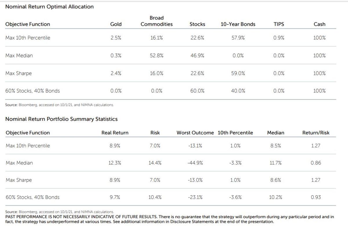
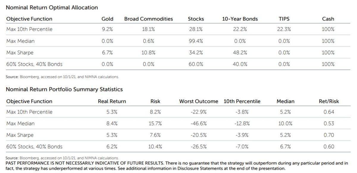
The calibration leads to a different set of real and nominal optimal portfolios for the same three objective functions described above. Some of the objective functions have similar optimal portfolios compared to before changing return expectations; others are quite different. Critically, all but the Max Median portfolio, which seeks to maximize median nominal returns with no consideration given to risk, have substantial allocations to broad commodities of between 12.1% and 19.2%. While average risk-adjusted returns across the optimal portfolios are lower compared to the historical optimal portfolios, there are still substantial returns available to savvy investors willing to allocate substantially to inflation-hedging assets. It is also interesting to notice that the most efficient portfolio in the real return space (Max Sharpe) has almost totally abandoned both nominal and real bonds and is instead getting diversification from gold and commodities. Furthermore, as expected, the allocation to gold is much more significant under the adjusted return history both because bonds are less attractive and because gold is assumed to offer better return than its longest history suggests.
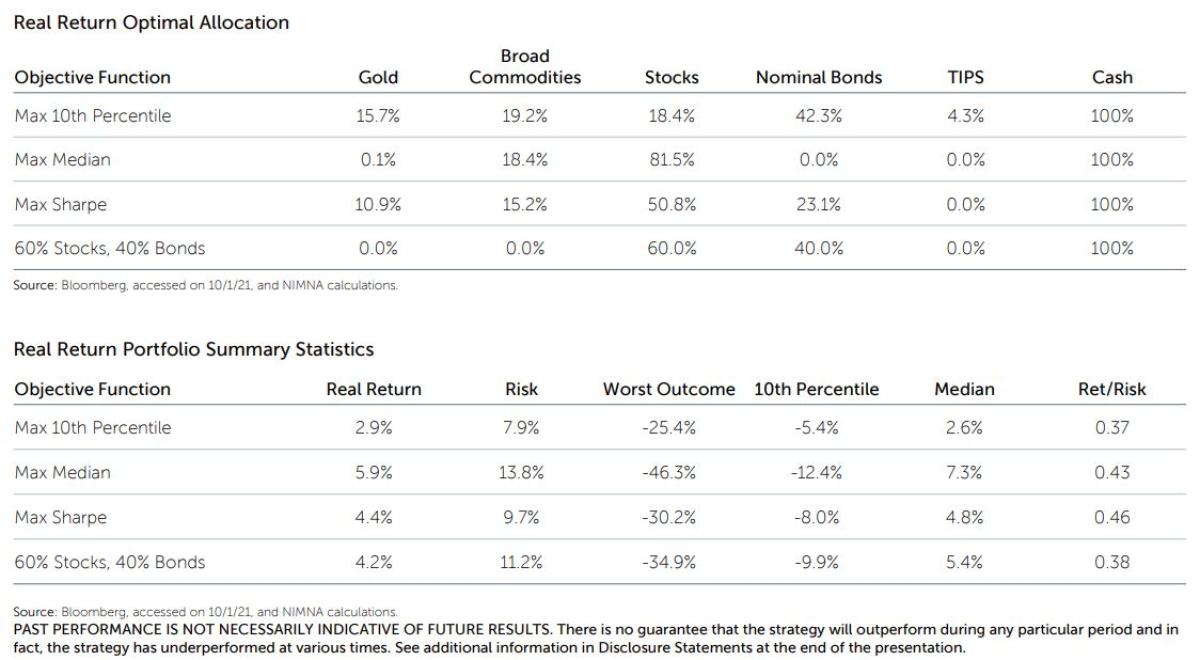
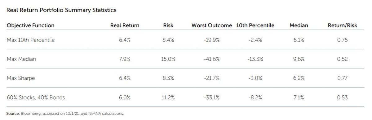
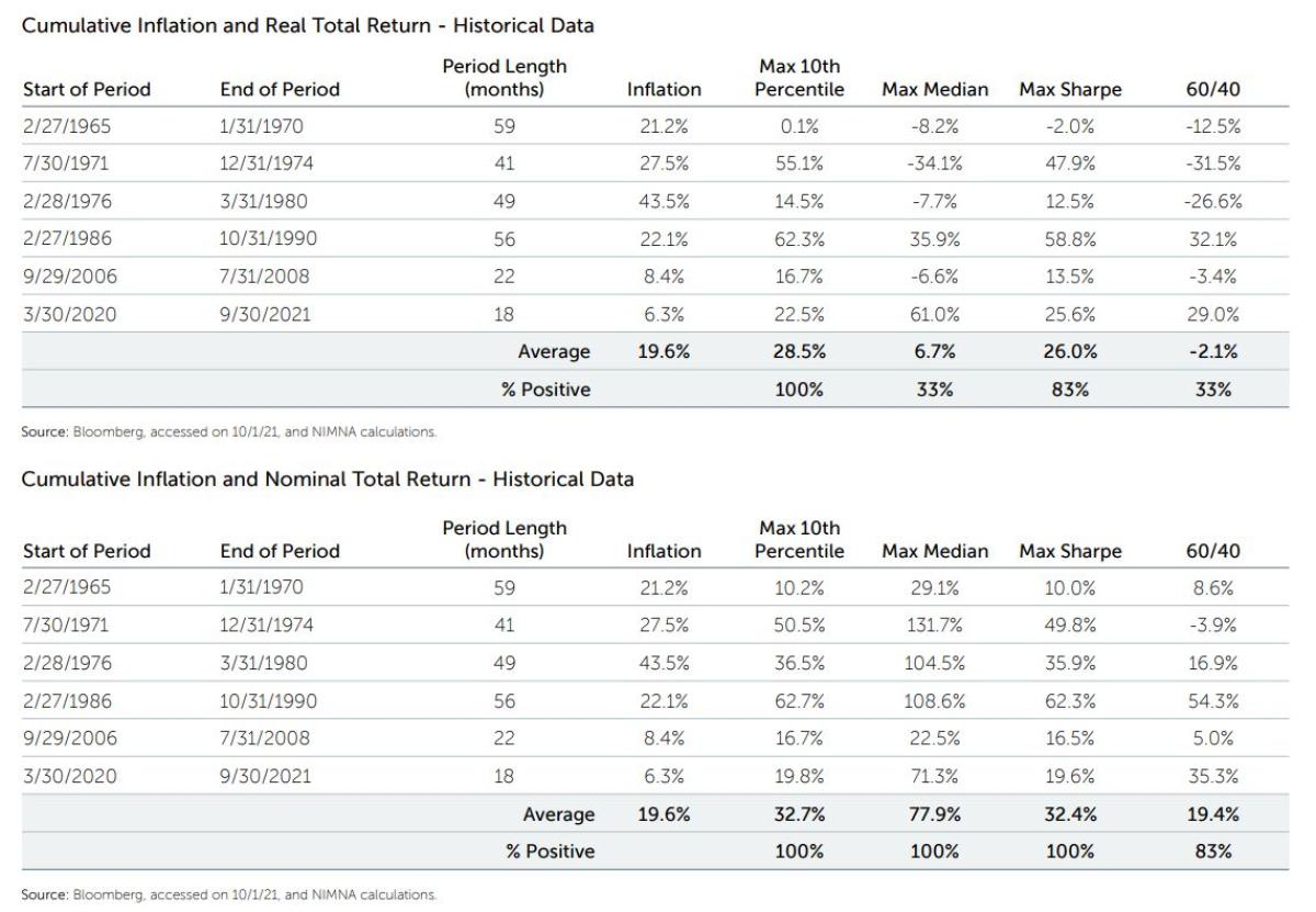
The table below shows the historical performance of the portfolios that were chosen as optimal based on our forward-looking return expectations during the historical inflation scenarios. The Max 10th Percentile and Max Sharpe portfolio objectives generate outcomes that are meaningfully more robust in inflation periods, with positive real returns 83% of the time, relative to 33% for 60% stocks/40% bonds. Nominal returns are positive 100% of the time, relative to 83% for 60/40, and the average performance during inflation periods is more than 12% higher.
To summarize the conclusions: regardless of objective function, virtually all investors would be well served by including an allocation to broad commodities from where we are today. Allocations to gold may be favorable depending on investor views and objectives. The non-negotiable portfolio tools are stocks and broad, intelligently implemented commodities. The future is likely to offer lower returns than the past, but a tilt modestly away from equities and bonds and toward broad, well-implemented commodities is still very likely to generate 5% real return or more in an efficient portfolio with reasonable risk. Nominal-return investors may still wish to deploy substantial capital in nominal bonds if they have the ability to modestly lever to reach for nominal returns of 7%, which would require about 40% leverage at the portfolio level but would preserve very manageable portfolio-level expected risk of about 11%—much less risk than would be required to deliver this return with a less diversified portfolio.
CONCLUSION
This paper examined the historical relationship between inflation and performance of stocks, bonds, and inflation-sensitive assets. We showed that broad commodities provided a more reliable hedge than gold during the periods when inflation was high and rising, and that TIPS hedged their own cash flows without providing much benefit to broader portfolios. The paper went on to show how one can use the well-known characteristics of commodity markets to build a portfolio with reasonable return/risk characteristics and with very high sensitivity to periods of inflation.
Because forward-looking bond returns are so poor, the opportunity cost of allocating to commodities is also very low. A commodity portfolio that can earn cash plus 3.5% in a benign environment and can also generate very high return if inflation rises becomes very attractive. As shown above, we believe real-return investors are particularly well served by commodity allocations on the order of 20%, funded out of the fixed-income allocation, and by shifting the remainder of their fixed-income allocation into TIPS.
Footnotes:
Note: 1 For simplicity, we use the Bloomberg Commodity 3 Months Forward Index (BCOM Index F3) to represent intelligently implemented commodities, as it captures most of the benefits of selecting optimal contract months for each commodity market. BCOM Index F3 is available starting in January 1991. We create a proxy for this series by taking the average difference between BCOMF3 and the front month BCOM Commodity Index over the period Jan 1991-August 2021 and adding it to the front month index for the entire time period January 1960-August 2021. This history for equity total return was extended back in time by adding a constant 4% dividend yield to price index returns prior to February 1988, when total return index observations become available.
Where “S&P 500” or ‘stocks’ are referenced, data for total returns begins in January 1988. Between 1971 and 1988, total return data is proxied by price return plus 1/12 of trailing 12-month dividend yield. Prior to 1971, S&P 500 total return is proxied by price return plus 3% per year. All data is from Bloomberg Finance LP. The S&P 500® Index and proxy are used to describe the performance of the large-cap segment of the US equity market.
We proxy 10-year bonds or nominal bonds by assuming that each month, the investor buys a new 10-year U.S. Treasury bond at face value for end-of-day yield for the last day of the prior month and simultaneously sells the prior month’s bond with 9 years and 11 months remaining to maturity, where the older bond is discounted by the current month yield. In addition, the bond investor earns 1/12 of the yield to maturity for the current month bond.
Data for “cash” is derived from the yield on 3-month US Treasury bills beginning in January 1954 and comes from Bloomberg Finance LP. Prior to that, we use data for the return on “cash” from the Ken French Data Library.
Data for the return on US 10-year TIPS begins in August 1998, which is totally inadequate for our purpose here of investigating the history of inflation hedging assets over several historical periods of high inflation. We solve this by using the data for TIPS that we do have and regressing the breakeven inflation rate implied by 10-year TIPS (breakeven inflation is the inflation rate at which an investor earns exactly the same return from nominal and inflation-protected bonds) on a constant and 3-, 12-, and 36-month inflation. We use this regression to create a fitted series for expected inflation which is then used to create a synthetic return series for inflation-linked bonds that starts in February 1962.
About the Author:
Roberto Croce Ph.D. is a Senior Portfolio Manager and Head of Liquid Alternatives at Newton Investment Management in Boston. In this role, Roberto and his team manage Newton's risk parity and risk premia offerings and design new strategies to solve clients' most pressing investment problems.
Prior to joining Newton in 2018, Roberto was the Head of Quantitative Strategies at Salient Partners in Houston. Rob joined Salient in 2011 as a quantitative analyst, early in Salient's transformation from a fund-of-funds manager into a direct manager of client assets. He led the build-out of quantitative infrastructure at Salient, eventually rising to Managing Director and Partner, as he managed a team of computer scientists, software engineers, and data scientists. The result was a fully automated investment process with a focus on empirical measurement and constant improvement of every facet of the investment process.
Prior to joining Salient Partners in 2011, Roberto spent six years at the Ohio State University teaching macroeconomics and econometrics. While at Ohio State, Rob spent a summer working on the Quantitative Research team at the Teachers Retirement System of Texas, where he had exposure to the application of financial theory to real-world institutional investing, with a particular focus on risk parity strategies.
Roberto has Ph.D. and MA degrees in economics from the Ohio State University and a BS in Business Economics from Penn State.